2.2 Governing Equations of Fiber Flow

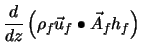
Mass conservation of a fiber element is written as

In this equation $\rho_f$ is the fiber density, $\vec{u}_f$ is the fiber velocity vector, $\vec{A}_f$ is the surface area vector of the fiber surface parallel to the flow direction, $Y_s$ is the mass fraction of the solvent $s$ in the fiber, $\dot{m}_s''$ is the evaporated mass flow rate of the solvent $s$, and $d_f$ is the fiber diameter. $\dot{m}_s''$ is calculated using a film theory.

The mass transfer coefficient $\beta$ is estimated from an appropriate correlation, see Section  2.8. $M_s$ is the solvent's molecular weight, $c$ is the molar concentration of the surrounding gas and $\psi_{s,g}$ is the mole fraction of the solvent vapor in the surrounding gas. At the fiber surface, the mole fraction of the solvent in the gas $\psi_{s,I}$ is related to the solvent mass fraction in the fiber $Y_s$ by the vapor-liquid equilibrium equation given by Flory [ 1],

where $\chi$ is the Flory-Huggins parameter, $p$ is the absolute pressure in the surrounding flow, and $p_{s,vap}$ is the saturation vapor pressure of the solvent. These equations are used only when dry spun fibers have been selected.

The formation of fibers is based on tensile forces in the fiber that are applied at the take-up point and result in the drawing and elongation of the fiber.

A force balance for a differential fiber element gives the equation of change of momentum in the fiber.

The tensile force in the fiber changes due to acceleration of the fiber, friction force with the surrounding gas, and the gravitational forces.

The friction force with the surrounding gas is computed by

where $\rho$ is the gas density, $c_{f,ax}$ is the axial friction factor parallel to the fiber, and $\vec{u}_{par}$ is the gas velocity parallel to the fiber.

The gravitational force is computed from

where $\vec{n}_f$ is the direction vector of the fiber element.

The tensile force $\vec{F}$ is related to the components of the stress tensor by

Neglecting visco-elastic effects and assuming Newtonian flow one can obtain

$$\tau_{zz} = 2 \eta_f \frac{d u_f}{d z}$$ (2.2-8)

$$\tau_{rr} = - \eta_f \frac{d u_f}{d z}$$ (2.2-9)

leading to

The elongational viscosity is estimated by multiplying the zero shear viscosity $\eta_f$ by three.

The transport of enthalpy in and to a differential fiber element is balanced to calculate the fiber temperature along the spinning line.

$$\frac{d}{dz} \left(\rho_f \vec{u}_f \bullet \vec{A}_f h_f\right) = \frac{d}{dz} \left( \lambda_f \vec{A}_f \frac{d T_f}{dz} \right) + \pi d_f \left( \alpha \left( T - T_f \right) - \dot{m}_{s}'' h_{s,v} \right)$$

$$+ \dot{Q}_{viscous heating}+ \dot{Q}_{radiation,abs} - \dot{Q}_{radiation, emission}$$ (2.2-11)

where $h_f$ is the fiber enthalpy, $\lambda_f$ is the fiber thermal conductivity, $T_f$ is the fiber temperature, $h_{s,v}$ is the enthalpy of the solvent vapor, and $\alpha$ is the heat transfer coefficient.

In the case of a melt spinning process, $\dot{m}_s''$ is zero since there is no mass transfer. The term for heat generation due to viscous heating is derived from the fluid mechanics of cylindrical flow to be

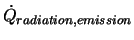
Radiation heat exchange is considered by the last two terms

$$\dot{Q}_{radiation,abs} = d_f \epsilon_f G$$ (2.2-13)

$$\dot{Q}_{radiation,emission} = \pi d_f \epsilon_f \sigma T_f^4$$ (2.2-14)

where $G$ is the thermal irradiation, $\epsilon_f$ is the fiber's emissivity, and $\sigma$ is the Boltzman constant.

The fiber enthalpy $h_f$ is related to the fiber temperature $T_f$ as follows

It uses $C_{{p}_{p}}$ the specific heat capacity of the polymer and $C_{{p}_{s}}$ the specific heat capacity of the solvent in the fiber.

The enthalpy of the solvent vapor at a given temperature $T_v$ depends on the heat of vaporization $\Delta h_s$, given at the vaporization temperature $T_{vap}$, and is computed from

where $C_{{p}_{s,l}}$ is the specific heat capacity of the solvent liquid and $C_{{p}_{s,v}}$ is the specific heat capacity of the solvent vapor.