16.5.14 Immiscible Fluid Model

The immiscible fluid model for Eulerian multiphase allows you to use the Geo-Reconstruct and CICSAM sharpening schemes with the explicict VOF option. This model should be enabled only for cases requiring sharp interface treatment between phases. This model might help in overcoming some limitations of the VOF model because of the shared velocity and temperature formulation.

The immiscible fluid model for the Eulerian multiphase model provides the anisotropic drag law, which can be used when modeling free surface flow. This drag law is also used when there is higher drag in the normal direction to the interface and lower drag in the tangential direction to the interface. This model may help in overcoming some limitations of the VOF model because of the shared velocity and temperature formulation.

In some cases, where the flow for a particular phase is important in both the directions (tangential and normal to the interface), using a higher anisotropy ratio will result in numerical instability. Therefore, in those cases, an anisotropy ratio of up to 1000 is recommended, where the anisotropy ratio is defined as

In cases, where flow for a particular phase is important only in one direction (tangential or normal to the interface), a higher anisotropy ratio could be used. The principal directions for this drag are based on the normal and tangential direction to the interface.

Two types of drag formulations exist within the anisotropic drag law: one that is based on the symmetric drag law and the other is based on different viscosity options.

Formulation 1

This is based on the symmetric drag law, where the effective drag coefficient in the principal direction $p$ is described as follows:

where $\lambda$ is the friction factor vector in the principal direction. $K_{symmetric}$ is the isotropic drag coefficient obtained from the symmetric drag law.

Formulation 2

The effective drag coefficient in the principal direction $p$ is described as follows:

where $vof_i$ is the volume fraction for phase $i$ and $vof_j$ is the volume fracion for phase $j$.

The viscous drag component in the principal direction $K_{visc},p$ is

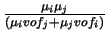
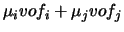
where the viscosity options can be any one of the following:

$\mu$	=	$0.5(\mu_i + \mu_j)$
$\mu$	=	$\frac{2 \mu_i \mu_j}{(\mu_i + \mu_j)}$
$\mu$	=	$\frac{\mu_i \mu_j}{(\mu_i vof_j + \mu_j vof_i)}$
$\mu$	=	$\mu_i vof_i + \mu_j vof_j$
$\mu$	=	$\mu_i$
$\mu$	=	$\mu_j$

and $l_c$ is the length scale.

To learn how to use the immiscible fluid model and the two drag formulations, refer to this section in the separate User's Guide.