2.2.2 Particle Birth and Death Due to Breakage and Aggregation

The birth and death of particles occur due to breakage and aggregation processes. Examples of breakage processes include crystal fracture in crystallizers and bubble breakage due to liquid turbulence in a bubble column. Similarly, aggregation can occur due to particle agglomeration in crystallizers and bubble coalescence in bubble column reactors.

Breakage

The breakage rate expression, or kernel [ 18], is expressed as

where

$g(V^\prime)$	=	breakage frequency; i.e., the fraction of particles of volume $V^\prime$ breaking
		per unit time (m $^{-3}$s $^{-1}$)
$\beta(V\mid V^\prime)$	=	probability density function (PDF) of particles breaking from volume
		$V^\prime$ to a particle of volume $V$

The birth rate of particles of volume $V$ due to breakage is given by

where 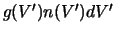$g(V^\prime)n(V^\prime)dV^{\prime}$ particles of volume $V^\prime$ break per unit time, producing 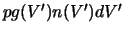$p g(V^\prime)n(V^\prime)d{V^\prime}$ particles, of which a fraction $\beta(V\mid V^\prime)dV$ represents particles of volume $V$. $p$ is the number of child particles produced per parent (e.g., two particles for binary breakage).

The death rate of particles of volume $V$ due to breakage is given by

The PDF $\beta(V\mid V^\prime)$ is also known as the particle fragmentation distribution function, or daughter size distribution. Several functional forms of the fragmentation distribution function have been proposed, though the following physical constraints must be met: the normalized number of breaking particles must sum to unity, the masses of the fragments must sum to the original particle mass, and the number of fragments formed has to be correctly represented.

Mathematically, these constraints can be written as follows:

• For the normalization condition:

  
  

  
  

• For conservation of mass

  
  

  
  

• For binary breakage, $\beta$ is symmetric about $V/V^{\prime} = 0.5$; i.e.,

  
  

  
  

The following is a list of models available in ANSYS FLUENT to calculate the breakage frequency:

• constant value

• Luo model

• Lehr model

• Ghadiri model

• user-defined model

ANSYS FLUENT provides the following models for calculating the breakage PDF:

• parabolic PDF

• generalized PDF for multiple breakage fragments

• user-defined model

The breakage frequency models and the parabolic and generalized PDFs are described in detail in the sections that follow.

Luo and Lehr Breakage Kernels

The Luo and Lehr models are integrated kernels, encompassing both the breakage frequency and the PDF of breaking particles. The general breakage rate per unit volume is usually written [ 15] as

where the original particle has a volume $V^{\prime}$ and the daughter particle has a volume $V$. In the previous expression, $\Omega_{\rm B} \left( V^{\prime} \right)$ is the breakage frequency, and $\eta \left( V \mid V^{\prime} \right)$ is the normalized daughter particle distribution function. For binary breakage, the breakage kernel must be symmetrical with respect to $\frac{V}{V^{\prime}} = 0.5$.

The general form is the integral over the size of eddies $\lambda$ hitting the particle with diameter $d$ (and volume $V$). The integral is taken over the dimensionless eddy size $\xi = \lambda / d$. The general form is

where the parameters are as shown in Table  2.2.1:

Table 2.2.1: Luo and Lehr Model Parameters

Ghadiri Breakage Kernels

The Ghadiri model [ 7, 22], in contrast to the Luo and Lehr models, is used to model only the breakage frequency of the solid particles. You will have to specify the PDF model to define the daughter distribution.

The breakage frequency $f$ is related to the material properties and impact conditions:

where $\rho_s$ is the particle density, $E$ is the elastic modulus of the granule, and $\Gamma$ is the interface energy. $v$ is the impact velocity and $L$ is the particle diameter prior to breaking. $K_b$ is the breakage constant and is defined as

Parabolic PDF

The breakage PDF function contains information on the probability of fragments formed by a breakage event. It provides the number of particles and the possible size distribution from the breakage. The parabolic form of the PDF implemented in ANSYS FLUENT allows you to define the breakage PDF such that

where $V$ and $V^\prime$ are the daughter and parent particle volumes, respectively. Depending on the value of the shape factor $C$, different behaviors will be observed in the shape of the particle breakage distribution function. For example, if $C = 2$, the particle breakage has a uniform distribution. If $0 < C < 2$, a concave parabola is obtained, meaning that it is more likely to obtain unequally-sized fragments than equally-sized fragments. The opposite of this is true for $2 < C < 3$. Values outside of the range of 0 to 3 are not allowed, because the PDF cannot have a negative value.

Note that the PDF defined in Equation  2.2-15 is symmetric about $V / V^\prime = 0.5$.

Generalized PDF

The generalized form of the PDF implemented in ANSYS FLUENT allows you to simulate multiple breakage fragments ( $>2$) and to specify the form of the daughter distribution (e.g., uniform, equisized, attrition, power law, parabolic, binary beta). The model itself can be applied to both the discrete method and the QMOM.

Considering the self-similar formulation [ 25] where the similarity $z$ is the ratio of daughter-to-parent size (i.e., $z \equiv \frac{V}{V^{\prime}}$), then the generalized PDF is given by

The $k^{\rm th}$ moment of $\theta (z)$ $(b_k)$ is

where

The conditions of number and mass conservation can then be expressed as

The generalized form of $\theta (z)$[ 6] can be expressed as

where $i$ can be 0 or 1, which represents $\theta (z)$ as consisting of 1 or 2 terms, respectively. For each term, $w_i$ is the weighting factor, $p_i$ is the averaged number of daughter particles, $q_i$ and $r_i$ are the exponents, and $\beta(q_i,r_i)$ is the beta function. The following constraints are imposed on the parameters in Equation  2.2-21:

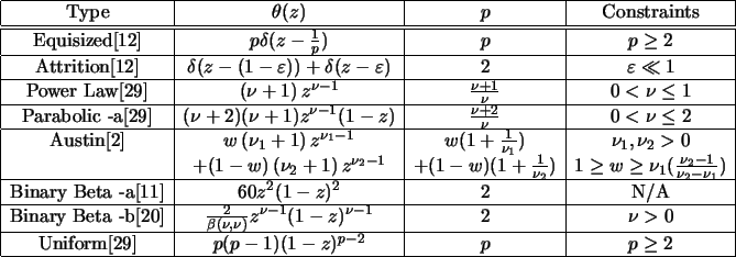
In order to demonstrate how to transform the generalized PDF to represent an appropriate daughter distribution, consider the expressions shown in Table  2.2.2:

Table 2.2.2: Daughter Distributions

In Table  2.2.2, $\delta$ is the Dirac delta function, $w$ is a weighting coefficient, and $\varepsilon$, $\nu$, $\nu_1$, and $\nu_2$ are user-defined parameters.

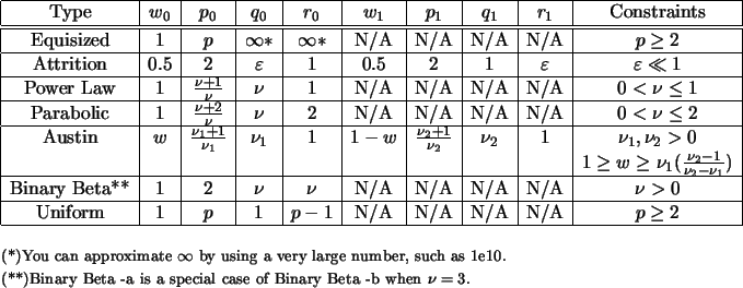
The generalized form can represent the daughter distributions in Table  2.2.2 by using the values shown in Table  2.2.3.

Table 2.2.3: Values for Daughter Distributions in General Form

Note that for the ANSYS FLUENT implementation of the generalized form of the PDF, you will only enter values for $w_0$, $p_0$, $q_0$, $r_0$, and $q_1$, and the remaining values ( $w_1$, $p_1$, and $r_1$) will be calculated automatically.

Aggregation

The aggregation kernel [ 18] is expressed as

The aggregation kernel has units of m $^3$/s, and is sometimes defined as a product of two quantities:

• the frequency of collisions between particles of volume $V$ and particles of volume $V^\prime$

• the "efficiency of aggregation'' (i.e., the probability of particles of volume $V$ coalescing with particles of volume $V^\prime$).

The birth rate of particles of volume $V$ due to aggregation is given by

where particles of volume $V-V^\prime$ aggregate with particles of volume $V^\prime$ to form particles of volume $V$. The factor $1/2$ is included to avoid accounting for each collision event twice.

The death rate of particles of volume $V$ due to aggregation is given by

The breakage and aggregation kernels depend on the nature of the physical application. For example, in gas-liquid dispersion, the kernels are functions of the local liquid-phase turbulent dissipation.

The following is a list of aggregation functions available in ANSYS FLUENT:

• constant

• Luo model

• Free molecular model

• Turbulent model

• user-defined model

The Luo, free molecular, and turbulent aggregation functions are described in detail in the sections that follow.

Luo Aggregation Kernel

For the Luo model [ 17], the general aggregation kernel is defined as the rate of particle volume formation as a result of binary collisions of particles with volumes $V_i$ and $V_j$:

where $\omega_{\rm ag} \left( V_i , V_j \right) [ {\rm m}^3 / {\rm sec} ]$ is the frequency of collision and $P_{\rm ag} \left( V_i , V_j \right)$ is the probability that the collision results in coalescence. The frequency is defined as follows:

where $\overline{u}_{i j}$ is the characteristic velocity of collision of two particles with diameters $d_i$ and $d_j$ and number densities $n_i$ and $n_j$. Two physical mechanisms are behind the calculation of this velocity. The first mechanism is turbulent mixing. Assuming that the particles' size lies in the inertial range of turbulence, and the turbulence is isotropic, the mixing velocity $\overline{u}_{i j}^t$ of the two particles can be expressed as

where

The expression for the probability of aggregation is

where $c_1$ is a constant of order unity, $x_{i j} = d_i / d_j$, $\rho_1$ and $\rho_2$ are the densities of the primary and secondary phases, respectively, and the Weber number is defined as

Free Molecular Aggregation Kernel

Real particles aggregate and break with frequencies (or kernels) characterized by complex dependencies over particle internal coordinates [ 28]. In particular, very small particles (say up to $1 \mu m$) aggregate because of collisions due to Brownian motions. In this case, the frequency of collision is size-dependent and usually the following kernel is implemented:

where $k_B$ is the Boltzmann constant, $T$ is the absolute temperature, $\mu$ is the viscosity of the suspending fluid. This kernel is also known as the Brownian kernel or the perikinetic kernel.

Turbulent Aggregation Kernel

During mixing processes, mechanical energy is supplied to the fluid. This energy creates turbulence within the fluid. The turbulence creates eddies, which in turn help dissipate the energy. The energy is transferred from the largest eddies to the smallest eddies in which it is dissipated through viscous interactions. The size of the smallest eddies is the Kolmogorov microscale, $\eta$, which is expressed as a function of the kinematic viscosity and the turbulent energy dissipation rate:

In the turbulent flow field, aggregation can occur by two mechanisms:

• viscous subrange mechanism: this is applied when particles are smaller than the Kolmogorov microscale, $\nu$

• inertial subrange mechanism: this is applied when particles are bigger than the Kolmogorov microscale. In this case, particles assume independent velocities.

For the viscous subrange, particle collisions are influenced by the local shear within the eddy. Based on work by Saffman and Turner [ 27], the collision rate is expressed as,

where $\varsigma_T$ is a pre-factor that takes into account the capture efficiency coefficient of turbulent collision, and $\dot{\gamma}$ is the shear rate:

For the inertial subrange, particles are bigger than the smallest eddy, therefore they are dragged by velocity fluctuations in the flow field. In this case, the aggregation rate is expressed using Abrahamson's model [ 1],

where $U_i^2$ is the mean squared velocity for particle $i$.

The empirical capture efficiency coefficient of turbulent collision describes the hydrodynamic and attractive interaction between colliding particles. Higashitani et al. [ 9] proposed the following relationship:

where $N_T$ is the ratio between the viscous force and the Van der Waals force,

Where $H$ is the Hamaker constant, a function of the particle material, and $\dot{\lambda}$ is the deformation rate,