Step 7: Solution

1.   Set the solution parameters.

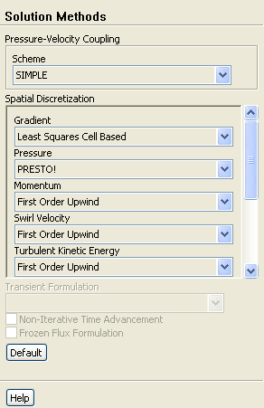
Solution Methods

(a)   Select PRESTO! from the Pressure drop-down list in the Spatial Discretization group box.

(b)   Retain the default selection of First Order Upwind for other parameters.

2.   Set the solution controls.

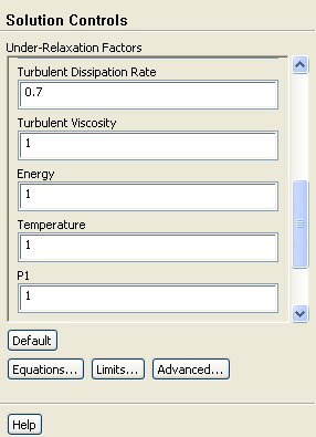
Solution Controls

(a)   Set the following parameters in the Under-Relaxation Factors group box:

Under-Relaxation Factor	Value
Pressure	0.5
Density	0.8
Momentum	0.3
Turbulent Kinetic Energy	0.7
Turbulent Dissipation Rate	0.7
P1	1

  The default under-relaxation factors are considered to be too aggressive for reacting flow cases with high swirl velocity.

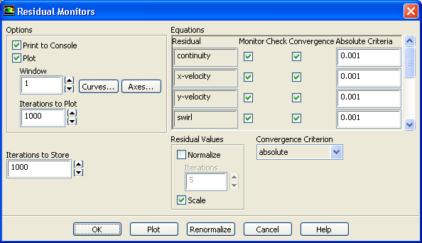
3.   Enable the display of residuals during the solution process.

Monitors Residuals Edit...

(a)   Ensure that the Plot is enabled in the Options group box.

(b)   Click OK to close the Residual Monitors dialog box.

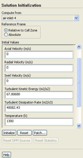
4.   Initialize the flow field using the conditions at air-inlet-4.

Solution Initialization

(a)   Select air-inlet-4 from the Compute from drop-down list.

(b)   Enter 0 m/s for Axial Velocity and Swirl Velocity.

(c)   Enter 1300 K for Temperature.

(d)   Click Initialize.

5.   Save the case file ( berl-1.cas.gz).

File $\rightarrow$ Write $\rightarrow$ Case...

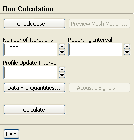
6.   Start the calculation by requesting 1500 iterations.

Run Calculation

  The solution will converge in approximately 1100 iterations.

7.   Save the first-order converged solution ( berl-1.dat.gz).

File $\rightarrow$ Write $\rightarrow$ Data...

8.   Switch to second-order upwind for improved accuracy.

Solution Methods

(a)   Ensure that PRESTO! is selected from the Pressure drop-down list in the Spatial Discretization group box.

(b)   Select Second Order Upwind for all the parameters except Mixture Fraction Variance.

9.   Save the case file ( berl-2.cas.gz).

File $\rightarrow$ Write $\rightarrow$ Case...

10.   Request an additional 800 iterations.

Run Calculation

  The solution will converge in approximately 720 iterations.

11.   Save the converged second-order flow data ( berl-2.dat.gz).

File $\rightarrow$ Write $\rightarrow$ Data...