Step 8: Postprocessing

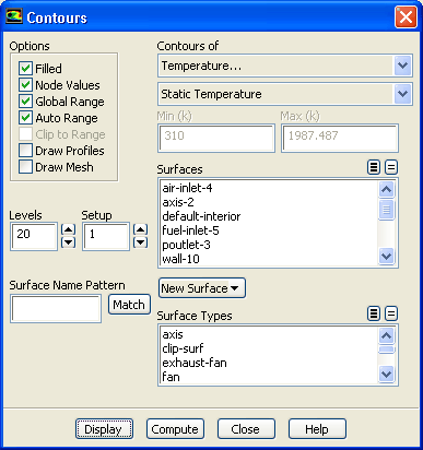
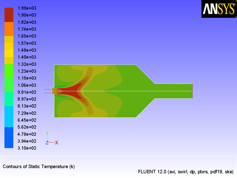
1.   Display the predicted temperature field (Figure  15.9).

Graphics and Animations Contours Set Up...

(a)   Enable Filled in the Options group box.

(b)   Select Temperature... and Static Temperature from the Contours of drop-down lists.

(c)   Click Display.

  The peak temperature in the system is 1987 K.

Figure 15.9: Temperature Contours

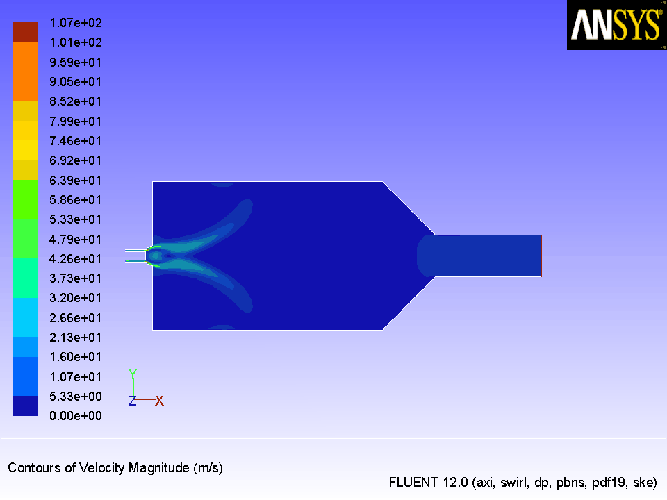
2.   Display contours of velocity (Figure  15.10).

Graphics and Animations Contours Set Up...

(a)   Select Velocity... and Velocity Magnitude from the Contours of drop-down lists.

(b)   Click Display.

Figure 15.10: Velocity Contours

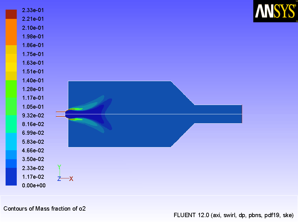
3.   Display the contours of mass fraction of o2 (Figure  15.11).

Graphics and Animations Contours Set Up...

(a)   Select Species... and Mass fraction of o2 from the Contours of drop-down lists.

(b)   Click Display and close the Contours dialog box.

Figure 15.11: Contours of Mass Fraction of o2