Step 8: Solution

1.   Set the solution parameters.

Solution Methods

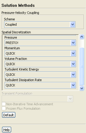
(a)   Select Coupled from the Scheme drop-down list in the Pressure-Velocity Coupling group box.

(b)   Select PRESTO! from the Pressure drop-down list in the Spatial Discretization group box.

(c)   Select QUICK for Momentum, Volume Fraction, Turbulent Kinetic Energy, and Turbulent Dissipation Rate.

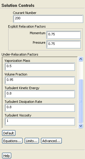
2.   Set the solution controls.

Solution Controls

(a)   Enter 0.5 for Vaporization Mass.

(b)   Enter 0.95 for Volume Fraction.

Note:    Typically, for more complex cases with very high pressure drops or large liquid-vapor density ratios, the under-relaxation factors may need to be reduced to between 0.1 and 0.2. For the Vaporization Mass, it is generally advised to use a value of 0.1, though this under-relaxation factor can be between 0.001 to 1 as necessary.

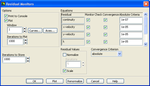
3.   Enable the plotting of residuals during the calculation.

Monitors Residuals Edit...

(a)   Ensure that Plot is enabled in the Options group box.

(b)   Enter 1e-07 for the Absolute Criteria of continuity.

(c)   Enter 1e-05 for the Absolute Criteria of x-velocity, y-velocity, k, and epsilon.

  Decreasing the criteria for these residuals will improve the accuracy of the solution.

(d)   Click OK to close the Residual Monitors dialog box.

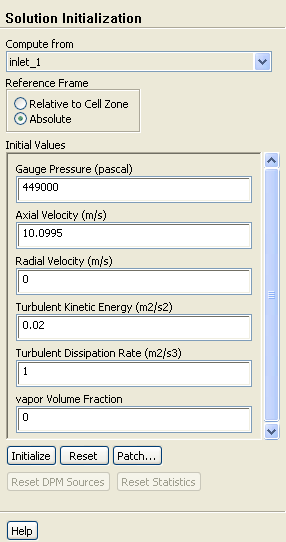
4.   Initialize the solution from either of the pressure inlet zones ( inlet_1 or inlet_2).

Solution Initialization

  

(a)   Select inlet_1 or inlet_2 from the Compute from drop-down list.

(b)   Select Absolute in the Reference Frame list.

(c)   Click Initialize to initialize the solution.

5.   Save the case file ( cav.cas.gz).

File $\rightarrow$ Write $\rightarrow$ Case...

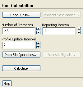
6.   Start the calculation by requesting 500 iterations.

Run Calculation

(a)   Enter 500 for Number of Iterations.

(b)   Click Calculate.

  The solution will converge in approximately 450 iterations.

7.   Save the data file ( cav.dat.gz).

File $\rightarrow$ Write $\rightarrow$ Data...