Step 9: Postprocessing

1.   Plot the pressure in the orifice (Figure  19.3).

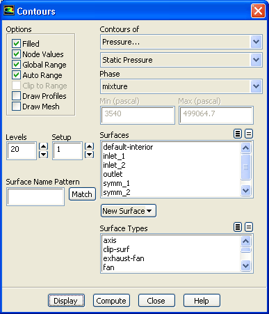
Graphics and Animations Contours Set Up...

(a)   Enable Filled in the Options group box.

(b)   Retain the default selection of Pressure... and Static Pressure from the Contours of drop-down lists.

(c)   Click Display and close the Contours dialog box.

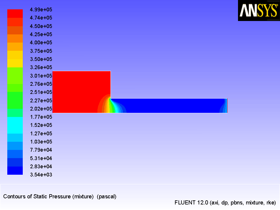
Figure 19.3: Contours of Static Pressure

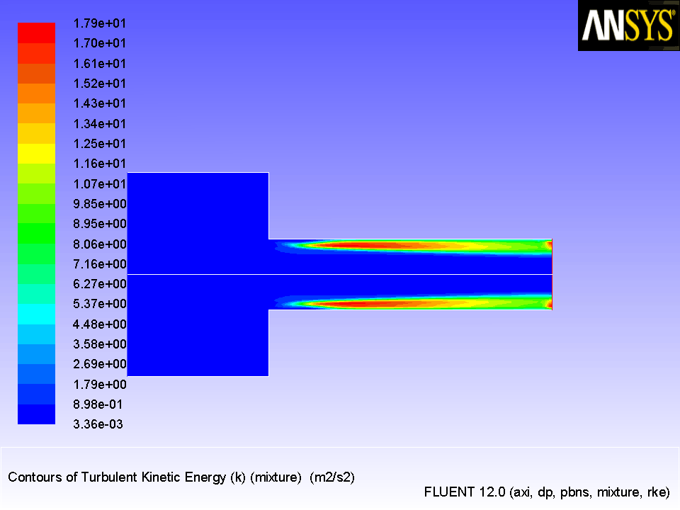
  Note the dramatic pressure drop at the flow restriction in Figure  19.3. Low static pressure is the major factor causing cavitation. Additionally, turbulence contributes to cavitation due to the effect of pressure fluctuation (Figure  19.4) and turbulent diffusion (Figure  19.5).

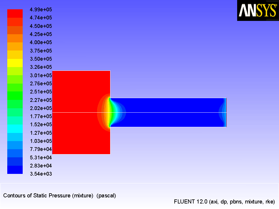
2.   Mirror the display across the centerline (Figure  19.4).

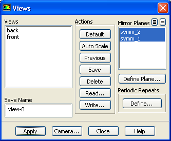
Graphics and Animations Views...

  Mirroring the display across the centerline gives a more realistic view.

(a)   Select symm_2 and symm_1 from the Mirror Planes selection list.

(b)   Click Apply and close the Views dialog box.

Figure 19.4: Mirrored View of Contours of Static Pressure

3.   Plot the turbulent kinetic energy (Figure  19.5).

Graphics and Animations Contours Set Up...

(a)   Select Turbulence... and Turbulent Kinetic Energy (k) from the Contours of drop-down lists.

(b)   Click Display.

Figure 19.5: Contours of Turbulent Kinetic Energy

  In this example, the mesh used is fairly coarse. However, in cavitating flows the pressure distribution is the dominant factor, and is not very sensitive to mesh size.

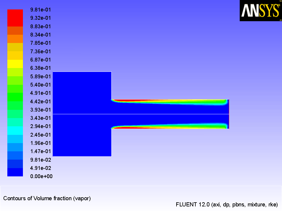
4.   Plot the volume fraction of water vapor (Figure  19.6).

Graphics and Animations Contours Set Up...

(a)   Select Phases... and Volume fraction from the Contours of drop-down lists.

(b)   Select vapor from the Phase drop-down list.

(c)   Click Display and close the Contours dialog box.

Figure 19.6: Contours of Vapor Volume Fraction

  The high turbulent kinetic energy region near the neck of the orifice in Figure  19.5 coincides with the highest volume fraction of vapor in Figure  19.6. This indicates the correct prediction of a localized high phase change rate. The vapor then gets convected downstream by the main flow.