Step 5: Postprocessing

  See Tutorial 1 for complete postprocessing exercises for this example. Here, two plots are generated so that you can confirm that the results obtained with the parallel solver are the same as those obtained with the serial solver.

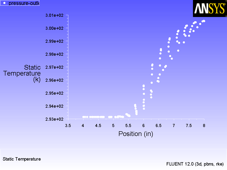
1.   Display an XY plot of temperature across the exit (Figure  26.4).

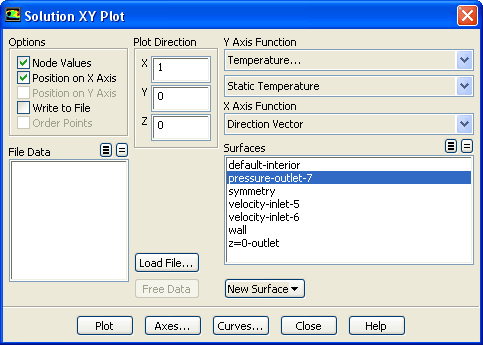
Plots XY Plot Set Up...

(a)   Select Temperature... and Static Temperature from the Y Axis Function drop-down lists.

(b)   Select pressure-outlet-7 from the Surfaces selection list.

(c)   Click Plot and close the Solution XY Plot dialog box.

Figure 26.4: Temperature Distribution at the Outlet

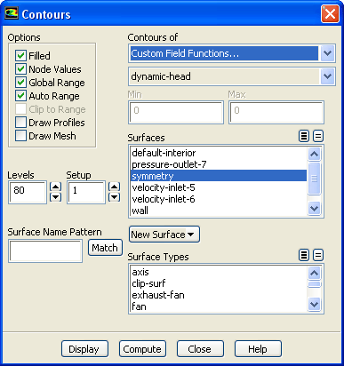
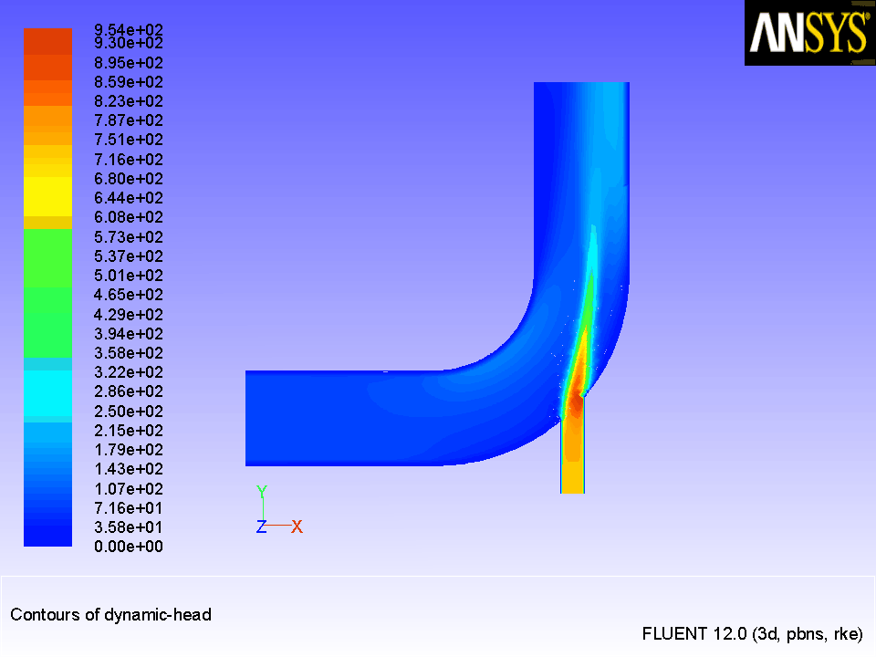
2.   Display filled contours of the custom field function dynamic-head (Figure  26.5).

Graphics and Animations Contours Set Up...

(a)   Select Custom Field Functions... from the Contours of drop-down list.

  The custom field function you created in Tutorial 1 ( dynamic-head) will be selected in the lower drop-down list.

(b)   Enter 80 for Levels.

(c)   Select symmetry from the Surfaces selection list.

(d)   Click Display and close the Contours dialog box.

Figure 26.5: Contours of the Custom Field Function, Dynamic Head