![[ANSYS, Inc. Logo]](fluentlogo.gif)


|
|
|
For liquid sprays, a convenient representation of the droplet size
distribution
is the Rosin-Rammler
expression. The complete range of sizes is divided into an adequate number of discrete intervals; each represented by a mean diameter for which trajectory calculations are performed. If the size distribution is of the Rosin-Rammler type, the mass fraction of droplets of diameter greater than
 is given by
where
 is the size constant and
 is the size distribution parameter.
By default, you will define the size distribution of particles by inputting a diameter for the first and last points and using the linear equation ( 23.3-1) to vary the diameter of each particle stream in the group. When you want a different mass flow rate for each particle/droplet size, however, the linear variation may not yield the distribution you need. Your particle size distribution may be defined most easily by fitting the size distribution data to the Rosin-Rammler equation. In this approach, the complete range of particle sizes is divided into a set of discrete size ranges, each to be defined by a single stream that is part of the group. Assume, for example, that the particle size data obeys the following distribution:
Diameter Range (
 m) m) |
Mass Fraction in Range |
| 0-70
70-100 100-120 120-150 150-180 180-200 |
0.05
0.10 0.35 0.30 0.15 0.05 |
The Rosin-Rammler distribution function is based on the assumption that an exponential relationship exists between the droplet diameter,
 , and the mass fraction of droplets with diameter greater than
 ,
,
 :
:
ANSYS FLUENT refers to the quantity
 in Equation
23.3-3 as the
Mean Diameter and to
in Equation
23.3-3 as the
Mean Diameter and to
 as the
Spread Parameter.
These parameters are input by you (in the
Set Injection Properties dialog box under the
First Point heading) to define the Rosin-Rammler size distribution. To solve for these parameters, you must fit your particle size data to the Rosin-Rammler exponential equation. To determine these inputs, first recast the given droplet size data in terms of the Rosin-Rammler format. For the example data provided above, this yields the following pairs of
as the
Spread Parameter.
These parameters are input by you (in the
Set Injection Properties dialog box under the
First Point heading) to define the Rosin-Rammler size distribution. To solve for these parameters, you must fit your particle size data to the Rosin-Rammler exponential equation. To determine these inputs, first recast the given droplet size data in terms of the Rosin-Rammler format. For the example data provided above, this yields the following pairs of
 and
and
 :
:
Diameter,
 ( (
 m) m) |
Mass Fraction with
Diameter Greater than  , ,
 |
| 70
100 120 150 180 200 |
0.95
0.85 0.50 0.20 0.05 (0.00) |
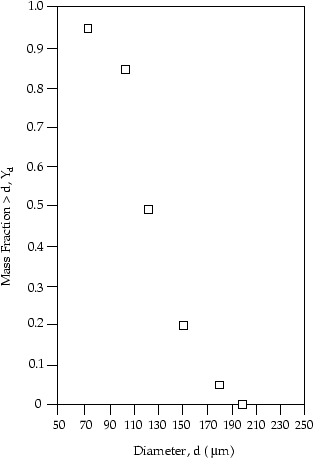
A plot of
 vs.
vs.
 is shown in Figure
23.3.6.
is shown in Figure
23.3.6.
Next, derive values of
 and
and
 such that the data in Figure
23.3.6 fit Equation
23.3-3. The value for
such that the data in Figure
23.3.6 fit Equation
23.3-3. The value for
 is obtained by noting that this is the value of
 at which
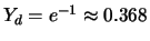 . From Figure
23.3.6, you can estimate that this occurs for
. From Figure
23.3.6, you can estimate that this occurs for

 m. The numerical value for
 is given by

By substituting the given data pairs for
 and
and
 into this equation, you can obtain values for
 and find an average. Doing so yields an average value of
 = 4.52 for the example data above. The resulting Rosin-Rammler curve fit is compared to the example data in Figure
23.3.7. You can input values for
= 4.52 for the example data above. The resulting Rosin-Rammler curve fit is compared to the example data in Figure
23.3.7. You can input values for
 and
and
 , as well as the diameter range of the data and the total mass flow rate for the combined individual size ranges, using the
Set Injection Properties dialog box.
, as well as the diameter range of the data and the total mass flow rate for the combined individual size ranges, using the
Set Injection Properties dialog box.
This technique of fitting the Rosin-Rammler curve to spray data is used when reporting the Rosin-Rammler diameter and spread parameter in the Discrete Phase Summary dialog box in Section 23.7.8.
A second Rosin-Rammler distribution is also available based on the natural logarithm of the particle diameter. If in your case, the smaller-diameter particles in a Rosin-Rammler distribution have higher mass flows in comparison with the larger-diameter particles, you may want better resolution of the smaller-diameter particle streams, or "bins''. You can therefore choose to have the diameter increments in the Rosin-Rammler distribution done uniformly by
 .
.
In the standard Rosin-Rammler distribution, a particle injection may have a diameter range of 1 to 200
 m. In the logarithmic Rosin-Rammler distribution, the same diameter range would be converted to a range of
 to
to
 , or about 0 to 5.3. In this way, the mass flow in one bin would be less-heavily skewed as compared to the other bins.
When a Rosin-Rammler size distribution is being defined for the group of streams, you should define (in addition to the initial velocity, position, and temperature) the following parameters, which appear under the heading for the First Point:
This is the total
mass flow rate of the
 streams in the group. Note that in axisymmetric problems this mass flow rate is defined per
 radians and in 2D problems per unit meter depth.
This is the smallest diameter to be considered in the size distribution.
This is the largest diameter to be considered in the size distribution.
This is the size parameter,
 , in the Rosin-Rammler equation (
23.3-3).
, in the Rosin-Rammler equation (
23.3-3).
This is the exponential parameter,
 , in Equation
23.3-3.
, in Equation
23.3-3.
The Stochastic Rosin-Rammler Diameter Distribution Method
For atomizer injections, a Rosin-Rammler distribution is assumed for the particles exiting the injector. In order to decrease the number of particles necessary to accurately describe the distribution, the diameter distribution function is randomly sampled for each instance where new particles are introduced into the domain.
The Rosin-Rammler distribution can be written as
![1-Y = \exp \left[ -\left(\frac{D}{\bar{d}} \right)^n \right]](img5527.gif) |
(23.3-4) |
 is the mass fraction smaller than a given diameter
 ,
,
 is the Rosin-Rammler diameter and
 is the Rosin-Rammler exponent. This expression can be inverted by taking logs of both sides and rearranging,
 along with parameters
 and
and
 , this function will explicitly provide a diameter,
 . Diameters for the atomizer injectors described in Section
23.3.7 are obtained by uniformly sampling
. Diameters for the atomizer injectors described in Section
23.3.7 are obtained by uniformly sampling
 in equation
23.3-5.
in equation
23.3-5.
Previous:
23.3.12 Point Properties for