![[ANSYS, Inc. Logo]](fluentlogo.gif)


|
|
|
At the center of the electrochemistry is the computation of the rates of the anodic and cathodic reactions. The electrochemistry model adopted in ANSYS FLUENT is the one that has been used by other groups ([ 3], [ 4], and [ 9]).
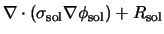
The driving force behind these reactions is the surface overpotential: the difference between the phase potential of the solid and the phase potential of the electrolyte/membrane. Therefore, two potential equations are solved for in the Fuel Cell and Electrolysis Model: one potential equation (Equation
1.2-1) accounts for the electron transport
 through the solid conductive materials (i.e., the current collectors and solid grids of the porous media); the other potential equation (
1.2-2) represents the protonic (i.e., ionic) transport of
through the solid conductive materials (i.e., the current collectors and solid grids of the porous media); the other potential equation (
1.2-2) represents the protonic (i.e., ionic) transport of
 or
or
 . The two potential equations are as follows:
where
 |
= | electrical conductivity (1/ohm-m) |
 |
= | electric potential (volts) |
 |
= | volumetric transfer current (
 ) ) |
The following figure illustrates the boundary conditions that are used to solve for
 and
and
 .
.
There are two types of external boundaries. Those through which there passes an electrical current and those through which there passes no current.
As no ionic current leaves the fuel cell through any external boundary, there is a zero flux boundary condition for the membrane phase potential,
 , on all outside boundaries.
For the solid phase potential,
 , there are external boundaries on the anode and the cathode side that are in contact with the external electric circuit and only through these boundaries passes the electrical current generated in the fuel cell. On all other external boundaries there is a zero flux boundary condition for
 .
.
On the external contact boundaries, we recommend to prescribe fixed values for
 (potentiostatic boundary conditions). If the anode side is set to zero, the (positive) value prescribed on the cathode side is the cell voltage. Specifying a constant flux (say on the cathode side) means to specify galvanostatic boundary conditions.
The transfer currents, or the source terms in Equations 1.2-1 and 1.2-2, are non-zero only inside the catalyst layers and are computed as:
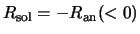 on the anode side and
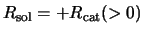 on the cathode side.
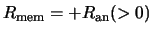 on the anode side and
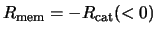 on the cathode side.
The source terms in Equations
1.2-1 and
1.2-2 (A/m
 ), have the following general definitions:
where
 |
= | reference exchange current density per active surface area (A/m
 ) ) |
 |
= | specific active surface area (1/m) |
![$[\;]$](img92.gif) , ,
![$[\;]_{\rm ref}$](img93.gif) |
= | local species concentration, reference value (kgmol/m
 ) ) |
 |
= | concentration dependence |
 |
= | transfer coefficient (dimensionless) |
 |
= | Faraday constant (
 C/kgmol) C/kgmol) |
The above equation is the general formulation of the Butler-Volmer function. A simplification to this is the Tafel formulation that reads,
By default, the Butler-Volmer function is used in the ANSYS FLUENT Fuel Cell and Electrolysis Model to compute the transfer currents inside the catalyst layers.
In Equations
1.2-3 through
1.2-6,
![$[A]$](img105.gif) and
and
![$[C]$](img106.gif) represent the molar concentration of the species upon which the anode and cathode reaction rates depend, respectively. For PEMFC and SOFC,
represent the molar concentration of the species upon which the anode and cathode reaction rates depend, respectively. For PEMFC and SOFC,
 represents
 and
and
 represents
 . For Electrolysis,
 represents
 and
and
 is 1.0 (which indicates that the cathode reaction does not depend on any species concentration).
The driving force for the kinetics is the local surface overpotential,
 , also known as the
activation loss. It is generally the difference between the solid and membrane potentials,
, also known as the
activation loss. It is generally the difference between the solid and membrane potentials,
 and
and
 .
.
The gain in electrical potential from crossing from the anode to the cathode side can then be taken into account by subtracting the open-circuit voltage
 on the cathode side.
From Equations 1.2-1 through 1.2-8, the two potential fields can be obtained.
Previous:
1.1.3 Introduction to Electrolysis





 and
and
 (PEMFC Used as an Example)


![$\displaystyle (\zeta_{\rm an} j^{\rm ref}_{\rm an}) \left(\frac{[A]}{[A]_{\rm... ...{\rm an} F \eta_{\rm an}/RT} - e^{-\alpha_{\rm cat} F \eta_{\rm an}/RT} \right)$](img85.gif)


![$\displaystyle (\zeta_{\rm cat} j^{\rm ref}_{\rm cat}) \left(\frac{[C]}{[C]_{\... ...rm an} F \eta_{\rm cat}/RT} + e^{-\alpha_{\rm cat} F \eta_{\rm cat}/RT} \right)$](img88.gif)


![$\displaystyle (\zeta_{\rm an} j^{\rm ref}_{\rm an}) \left(\frac{[A]}{[A]_{\rm ... ...\right)^{\gamma_{\rm an}} \left(e^{\alpha_{\rm an} F \eta_{\rm an}/RT} \right)$](img101.gif)


![$\displaystyle (\zeta_{\rm cat} j^{\rm ref}_{\rm cat}) \left(\frac{[C]}{[C]_{\r... ...ht)^{\gamma_{\rm cat}} \left(e^{-\alpha_{\rm cat} F \eta_{\rm cat}/RT} \right)$](img104.gif)

