2.3.1 The Discrete Method

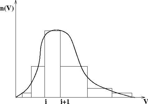
The discrete method (also known as the classes or sectional method) was developed by Hounslow [ 10], Litster [ 16], and Ramkrishna [ 25]. It is based on representing the continuous particle size distribution (PSD) in terms of a set of discrete size classes or bins, as illustrated in Figure  2.3.1. The advantages of this method are its robust numerics and that it gives the PSD directly. The disadvantages are that the bins must be defined a priori and that a large number of classes may be required.

Figure 2.3.1: A Particle Size Distribution as Represented by the Discrete Method

Numerical Method

In ANSYS FLUENT, the PBE is written in terms of volume fraction of particle size $i$:

where $\rho_s$ is the density of the secondary phase and $\alpha_i$ is the volume fraction of particle size $i$, defined as

where

and $V_i$ is the volume of the particle size $i$. In ANSYS FLUENT, a fraction of $\alpha$, called $f_i$, is introduced as the solution variable. This fraction is defined as

where $\alpha$ is the total volume fraction of the secondary phase.

The nucleation rate $\dot{n}_0$ appears in the discretized equation for the volume fraction of the smallest size $V_0$. The notation $0^i$ signifies that this particular term, in this case $\rho_s V_0 \dot{n}_0$, appears in Equation  2.3-1 only in the case of the smallest particle size.

The growth rate in Equation  2.3-1 is discretized as follows [ 10]:

The volume coordinate is discretized as [ 10] 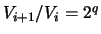$V_{i+1}/V_{i} = 2^{q}$ where $q = 1, 2,\ldots$ and is referred to as the "ratio factor''.

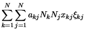
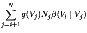
The particle birth and death rates are defined as follows:

$$B_{{\rm ag},i} = \sum_{k=1}^N \sum_{j=1}^N a_{kj} N_k N_j x_{kj} \xi_{kj}$$ (2.3-6)

$$D_{{\rm ag},i} = \sum_{j=1}^N a_{ij} N_i N_j$$ (2.3-7)

$$B_{{\rm br},i} = \sum_{j=i+1}^N g(V_j) N_j \beta(V_i \mid V_j)$$ (2.3-8)

$$D_{{\rm br},i} = g(V_i) N_i$$ (2.3-9)

where 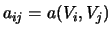$a_{ij} = a(V_i,V_j)$ and

$V_{\rm ag}$ is the particle volume resulting from the aggregation of particles $k$ and $j$, and is defined as

where

If $V_{\rm ag}$ is greater than or equal to the largest particle size $V_N$, then the contribution to class $N-1$ is

Note that there is no breakage for the smallest particle class.

Breakage Formulations for the Discrete Method

The default breakage formulation for the discrete method in ANSYS FLUENT is based on the Hagesather method [ 14]. In this method, the breakage sources are distributed to the respective size bins, preserving mass and number density. For the case when the ratio between successive bin sizes can be expressed as $2^n$ where $n=1,2,\ldots$, the source in bin $i$, ( $i=1,\ldots, N$) can be expressed as

Here

A more mathematically rigourous formulation is given by Ramakrishna [ 13], where the breakage rate is expressed as

where

The Ramakrishna formulation can be slow due to the large number of integration points required. However, for simple forms of $\beta$, the integrations can be performed relatively easily. The Hagesather formulation requires fewer integration points and the difference in accuracy with the Ramakrishna formulation can be corrected by a suitable choice of bin sizes.

To keep the computing time reasonable, a volume averaged value is used for the turbulent eddy dissipation when the Luo model is used in conjunction with the Ramakrishna formulation.