[ANSYS, Inc. Logo] return to home search
next up previous contents

Step 6: Solution: Steady Flow

  In this step, you will generate a steady-state flow solution that will be used as an initial condition for the time-dependent solution.

1.   Set the solution parameters.

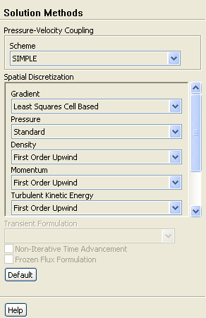
figure Solution Methods

figure

(a)   Retain all default discretization schemes in the Solution Methods task page.

  This problem has been found to converge satisfactorily with these default settings.

2.   Set the relaxation factors.

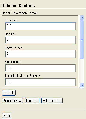
figure Solution Controls

figure

(a)   Retain the default values for Under-Relaxation Factors in the Solution Controls task page.

3.   Enable the plotting of residuals during the calculation.

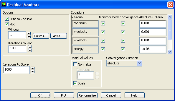
figure Monitors figure figure Residuals figure Edit...

figure

(a)   Make sure Plot is enabled in the Options group box.

(b)   Click OK to close the Residual Monitors dialog box.

4.   Initialize the solution.

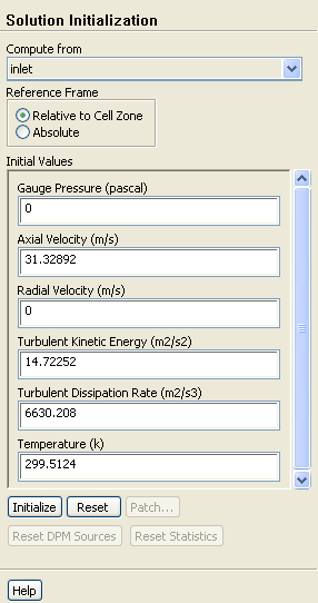
figure Solution Initialization

figure

(a)   Select inlet from the Compute From drop-down list.

(b)   Click Initialize in the Solution Initialization task page.

5.   Save the case file ( valve_init.cas.gz).

File $\rightarrow$ Write $\rightarrow$ Case...

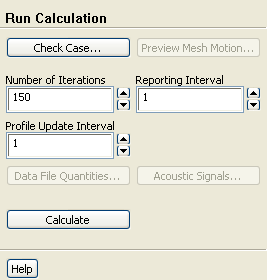
6.   Start the calculation by requesting 150 iterations.

figure Run Calculation

figure

  The solution converges in approximately 100 iterations.

7.   Save the case and data files ( valve_init.cas.gz and valve_init.dat.gz).

File $\rightarrow$ Write $\rightarrow$ Case & Data...


next up previous contents Previous: Step 5: Boundary Conditions
Up: Using Dynamic Meshes
Next: Step 7: Time-Dependent Solution
Release 12.0 © ANSYS, Inc. 2009-02-09