Step 8: Mesh Motion

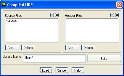
1.   Select and compile the user-defined function (UDF).

Define $\rightarrow$ User-Defined $\rightarrow$ Functions $\rightarrow$ Compiled...

  

(a)   Click Add... in the Source Files group box.

  The Select File dialog box will open.

i.   Select the source code valve.c in the Select File dialog box, and click OK.

(b)   Click Build in the Compiled UDFs dialog box.

  The UDF has already been defined, but it needs to be compiled within ANSYS FLUENT before it can be used in the solver. Here you will create a library with the default name of libudf in your working folder. If you would like to use a different name, you can enter it in the Library Name field. In this case you need to make sure that you will open the correct library in the next step.

  A dialog box will appear warning you to make sure that the UDF source files are in the folder that contains your case and data files. Click OK in the warning dialog box.

(c)   Click Load to load the UDF library you just compiled.

  When the UDF is built and loaded, it is available to hook to your model. Its name will appear as valve::libudf and can be selected from drop-down lists of various dialog boxes.

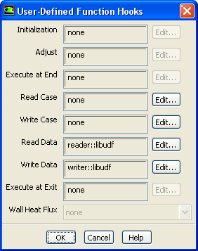
2.   Hook your model to the UDF library.

Define $\rightarrow$ User-Defined $\rightarrow$ Function Hooks...

(a)   Click the Edit... button next to Read Data to open the Read Data Functions dialog box.

i.   Select reader::libudf from the Available Read Data Functions selection list.

ii.   Click Add to add the selected function to the Selected Read Data Functions selection list.

iii.   Click OK to close the Read Data Functions dialog box.

(b)   Click the Edit... button next to Write Data to open the Write Data Functions dialog box.

i.   Select writer::libudf from the Available Write Data Functions selection list.

ii.   Click Add to add the selected function to the Selected Write Data Functions selection list.

iii.   Click OK to close the Write Data Functions dialog box.

  These two functions will read/write the position of C.G. and velocity in the X direction to the data file. The location of C.G. and the velocity are necessary for restarting a case. When starting from an intermediate case and data file, ANSYS FLUENT needs to know the location of C.G. and velocity, which are the initial conditions for the motion calculation. Those values are saved in the data file using the writer UDF and will be read in using the reader UDF when reading the data file.

(c)   Click OK to close the User-Defined Function Hooks dialog box.

3.   Enable dynamic mesh motion and specify the associated parameters.

Dynamic Mesh

(a)   Enable Dynamic Mesh in the Dynamic Mesh task page.

For more information on the available models for moving and deforming zones, see this chapter in the separate User's Guide.

(b)   Disable Smoothing and enable Layering in the Mesh Methods group box.

   ANSYS FLUENT will automatically flag the existing mesh zones for use of the different dynamic mesh methods where applicable.

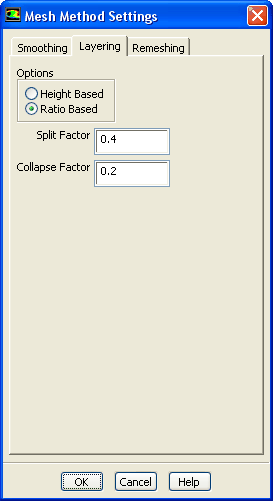
(c)   Click the Settings... button to open the Mesh Method Settings dialog box.

i.   Click the Layering tab.

ii.   Select Ratio Based in the Options group box.

iii.   Retain the default settings of 0.4 and 0.2 for Split Factor and Collapse Factor, respectively.

iv.   Click OK to close the Mesh Method Settings dialog box.

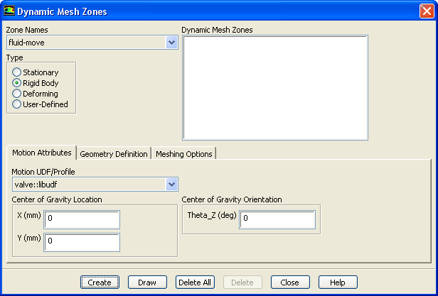
4.   Specify the motion of the fluid region ( fluid-move).

Dynamic Mesh Create/Edit...

  The valve motion and the motion of the fluid region are specified by means of the UDF valve.

(a)   Select fluid-move from the Zone Names drop-down list.

(b)   Retain the default selection of Rigid Body in the Type group box.

(c)   Make sure that valve::libudf is selected from the Motion UDF/Profile drop-down list in the Motion Attributes tab to hook the UDF to your model.

(d)   Retain the default settings of (0, 0) m for Center of Gravity Location, and 0 for Center of Gravity Orientation.

  Specifying the C.G. location and orientation is not necessary in this case, because the valve motion and the initial C.G. position of the valve are already defined by the UDF.

(e)   Click Create.

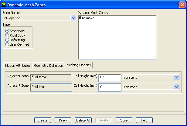
5.   Specify the meshing options for the stationary layering interface ( int-layering) in the Dynamic Mesh Zones dialog box.

(a)   Select int-layering from the Zone Names drop-down list.

(b)   Select Stationary in the Type group box.

(c)   Click the Meshing Options tab.

i.   Enter 0.5 mm for Cell Height of the fluid-move Adjacent Zone.

ii.   Retain the default value of 0 mm for the Cell Height of the fluid-inlet Adjacent zone.

(d)   Click Create.

6.   Specify the meshing options for the stationary outlet ( outlet) in the Dynamic Mesh Zones dialog box.

(a)   Select outlet from the Zone Names drop-down list.

(b)   Retain the previous selection of Stationary in the Type group box.

(c)   In the Meshing Options tab and enter 1.9 mm for the Cell Height of the fluid-move Adjacent Zone.

(d)   Click Create.

7.   Specify the meshing options for the stationary seat valve ( seat-valve) in the Dynamic Mesh Zones dialog box.

(a)   Select seat-valve from the Zone Names drop-down list.

(b)   Retain the previous selection of Stationary in the Type group box.

(c)   In the Meshing Options tab and enter 0.5 mm for Cell Height of the fluid-move Adjacent Zone.

(d)   Click Create.

8.   Specify the motion of the valve ( valve) in the Dynamic Mesh Zones dialog box.

(a)   Select valve from the Zone Names drop-down list.

(b)   Select Rigid Body in the Type group box.

(c)   Click the Motion Attributes tab.

i.   Make sure that valve::libudf is selected from the Motion UDF/Profile drop-down list to hook the UDF to your model.

ii.   Retain the default settings of (0, 0) m for Center of Gravity Location, and 0 for Center of Gravity Orientation.

(d)   Click the Meshing Options tab and enter 0 mm for the Cell Height of the fluid-move Adjacent zone.

(e)   Click Create and close the Dynamic Mesh Zones dialog box.

  In many MDM problems, you may want to preview the mesh motion before proceeding. In this problem, the mesh motion is driven by the pressure exerted by the fluid on the valve and acting against the inertia of the valve. Hence, for this problem, mesh motion in the absence of a flow field solution is meaningless, and you will not use this feature here.