Step 9: Time-Dependent Solution

1.   Set the solution paramters.

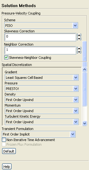
Solution Methods

(a)   Select PISO from the Scheme drop-down list in Pressure-Velocity Coupling group box.

(b)   Enter 0 for Skewness Correction.

(c)   Select PRESTO! from the Pressure drop-down list in the Spatial Discretization group box.

2.   Set the relaxation factors.

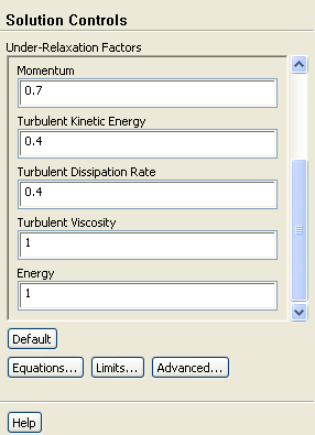
Solution Controls

(a)   Enter 0.6 for Pressure in the Under-Relaxation Factors group box.

(b)   Enter 0.4 for Turbulent Kinetic Energy and Turbulent Dissipation Rate in the Under-Relaxation Factors group box.

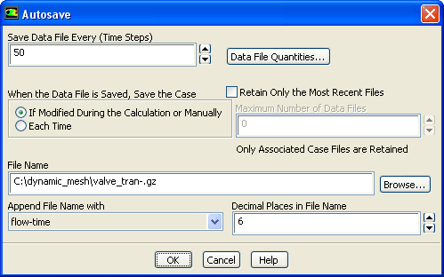
3.   Request that case and data files are automatically saved every 50 time steps.

Calculation Activities ( Autosave Every (Time Steps)) Edit...

(a)   Enter 50 for Save Data File Every (Time Steps).

(b)   Enter valve_tran-.gz in the File Name text box.

(c)   Select flow-time from the Append File Name with drop-down list.

  When ANSYS FLUENT saves a file, it will append the flow time value to the file name prefix ( valve_tran-). The gzipped standard extensions ( .cas.gz and .dat.gz) will also be appended.

(d)   Click OK to close the Autosave dialog box.

4.   Create animation sequences for the static pressure contour plots and velocity vectors plots for the valve.

Calculation Activities ( Solution Animations) Create/Edit...

  Use the solution animation feature to save contour plots of temperature every five time steps. After the calculation is complete, you use the solution animation playback feature to view the animated temperature plots over time.

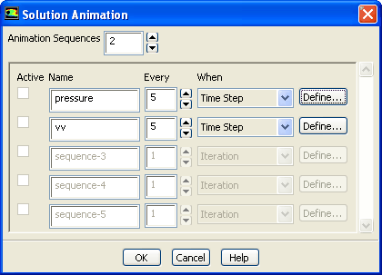
(a)   Set Animation Sequences to 2.

(b)   Enter pressure in the Name text box for the first animation.

(c)   Enter vv in the Name text box for the second animation.

(d)   Set Every to 5 for both animation sequences.

  The default value of 1 instructs ANSYS FLUENT to update the animation sequence at every time step. For this case, this would generate a large number of files.

(e)   Select Time Step from the When drop-down list for pressure and vv.

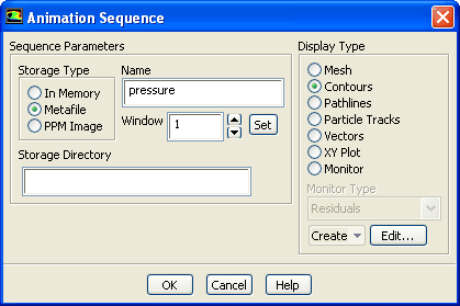
(f)   Click the Define... button next to pressure to open the Animation Sequence dialog box.

i.   Retain the default selection of Metafile in the Storage Type group box.

Note:   If you want to store the plots in a folder other than your working folder, enter the folder path in the Storage Directory text box. If this field is left blank (the default), the files will be saved in your working folder (i.e., the folder where you started ANSYS FLUENT).

ii.   Set Window number to 1 and click Set.

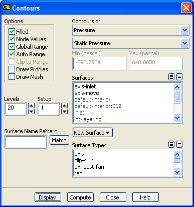
iii.   Select Contours in the Display Type group box to open the Contours dialog box.

a.   Enable Filled in the Options group box.

b.   Retain the default selection of Pressure... and Static Pressure from the Contours of drop-down lists.

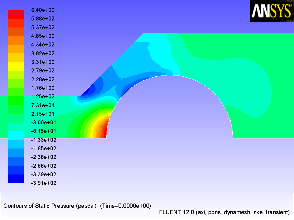
c.   Click Display (Figure  13.3).

Figure 13.3: Contours of Static Pressure at $t=0$ s

d.   Close the Contours dialog box.

iv.   Click OK in the Animation Sequence dialog box.

  The Animation Sequence dialog box will close, and the checkbox in the Active column next to pressure in the Solution Animation dialog box will be enabled.

(g)   Click the Define... button next to vv to open the Animation Sequence dialog box.

i.   Retain the default selection of Metafile in the Storage Type group box.

ii.   Set Window to 2 and click Set.

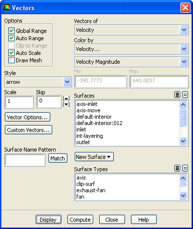
iii.   Select Vectors in the Display Type group box to open the Vectors dialog box.

a.   Retain all the default settings.

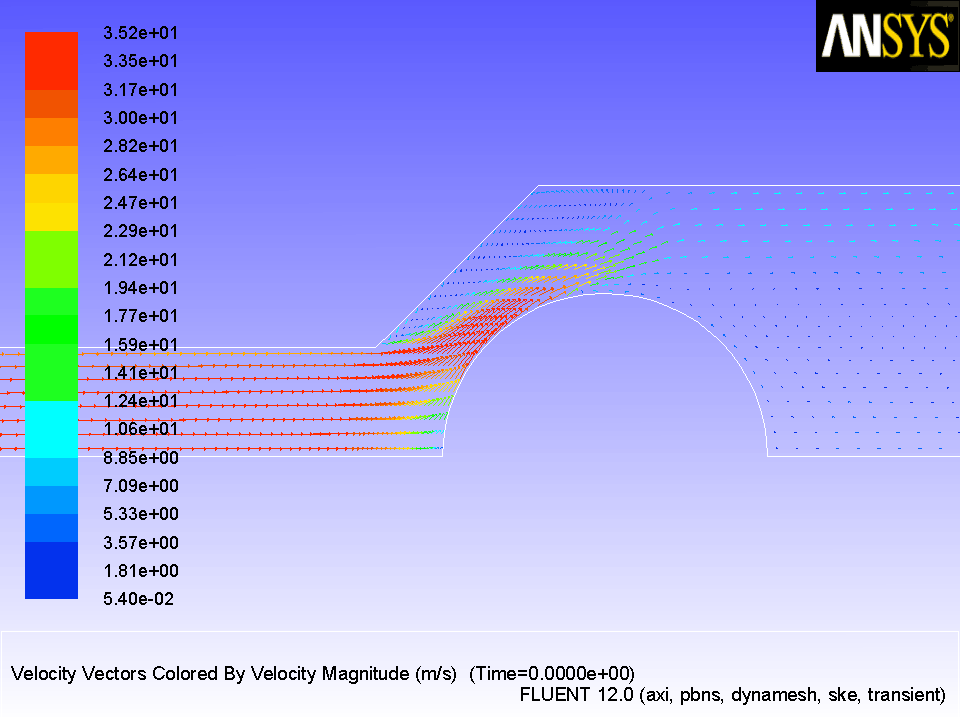
b.   Click Display (Figure  13.4).

Figure 13.4: Vectors of Velocity at $t=0$ s

c.   Close the Vectors dialog box.

iv.   Click OK in the Animation Sequence dialog box.

  The Animation Sequence dialog box will close, and the checkbox in the Active column next to vv in the Solution Animation dialog box will be enabled.

(h)   Click OK to close the Solution Animation dialog box.

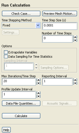
5.   Set the time step parameters for the calculation.

Run Calculation

(a)   Enter 0.0001 s for Time Step Size.

(b)   Retain 20 for Max Iterations/Time Step.

  In the accurate solution of a real-life time-dependent CFD problem, it is important to make sure that the solution converges at every time step to within the desired accuracy. Here the first few time steps will only come to a reasonably converged solution.

  This will save the time step size to the case file (the next time a case file is saved).

6.   Save the initial case and data files for this transient problem ( valve_tran-0.000000.cas.gz and valve_tran-0.000000.dat.gz).

File $\rightarrow$ Write $\rightarrow$ Case & Data...

7.   Request 150 time steps.

Run Calculation

Extra:   If you decide to read in the case file that is provided for this tutorial on the documentation CD, you will need to compile the UDF associated with this tutorial in your working folder. This is necessary because ANSYS FLUENT will expect to find the correct UDF libraries in your working folder when reading the case file.

The UDF (valve.c) that is provided can be edited and customized by changing the parameters as required for your case. In this tutorial, the values necessary for this case were preset in the source code. These values may be modified to best suit your model.