- 1.
Enable the NOx model.
 Models

 NOx
NOx
 Edit...
- (a)
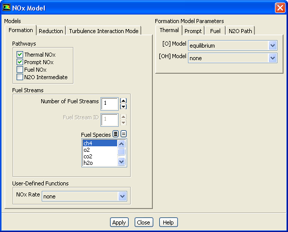
Enable
Thermal NOx
and
Prompt NOx in the
Pathways group box.
- (b)
Select
ch4 from the
Fuel Species selection list.
- (c)
Click the
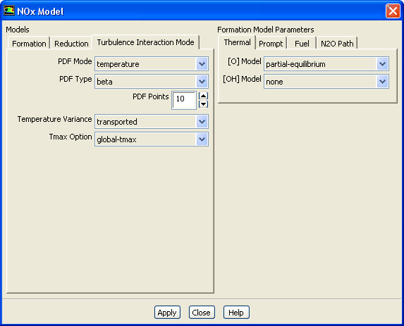
Turbulence Interaction Mode tab.
- i.
Select
temperature from the
PDF Mode drop-down list.
-
This will enable the turbulence-chemistry interaction.
If turbulence interaction is not enabled, you will be computing NOx formation without considering the important influence of turbulent fluctuations on the time-averaged reaction rates.
- ii.
Retain the default selection of
beta from the
PDF Type drop-down list and the default value of
10 for
PDF Points.
-
You can increase the value for
PDF Points to obtain a more accurate NOx prediction.
- iii.
Select
transported from the
Temperature Variance drop-down list.
- (d)
Select
partial-equilibrium from the
[O] Model drop-down list in the
Formation Model Parameters group box in the
Thermal tab.
-
The partial-equilibrium model
is used to predict the O radical concentration required for thermal NOx prediction.
- (e)
Click the
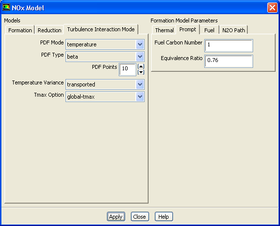
Prompt tab.
- i.
Retain the default value of
1 for
Fuel Carbon Number.
- ii.
Enter
0.76 for
Equivalence Ratio.
-
All of the parameters in the
Prompt tab are used in the calculation of prompt NOx formation. The
Fuel Carbon Number is the number of carbon atoms per molecule of fuel. The
Equivalence Ratio defines the fuel-air ratio (relative to stoichiometric conditions).
- (f)
Click
Apply to accept these changes and close the
NOx Model dialog box.
- 2.
Enable the calculation of NO species only and temperature variance.
 Solution Controls
 Equations...
- (a)
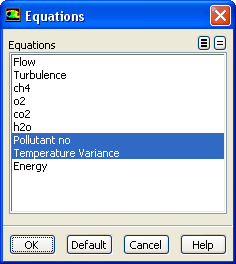
Deselect all variables except
Pollutant no and
Temperature Variance from the
Equations selection list.
- (b)
Click
OK to close the
Equations dialog box.
- 3.
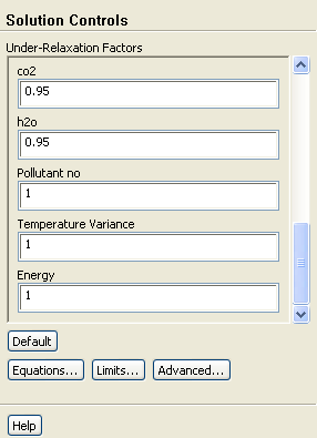
Set the under-relaxation factor for
Pollutant no.
 Solution Controls
- (a)
Enter
1 for
Pollutant no and
Temperature Variance in the
Under-Relaxation Factors group box.
-
You will predict NOx formation in a "postprocessing'' mode, with the flow field, temperature, and hydrocarbon combustion species concentrations fixed. Hence, only the NO equation will be computed. Prediction of NO in this mode is justified on the grounds that the NO concentrations are very low and have negligible impact on the hydrocarbon combustion prediction.
- 4.
Reduce the convergence criterion for the NO species equation.
 Monitors

 Residuals
 Edit...
- (a)
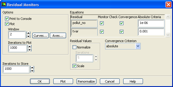
Ensure that the
Absolute Criteria for
pollut_no is set to
1e-06.
- (b)
Click
OK to close the
Residual Monitors dialog box.
- 5.
Request 50 more iterations.
 Run Calculation
-
The solution will converge in approximately 10 iterations.
- 6.
Save the new case and data files (
gascomb3.cas.gz and
gascomb3.dat.gz).
File
 Write
Write
 Case & Data...
- 7.
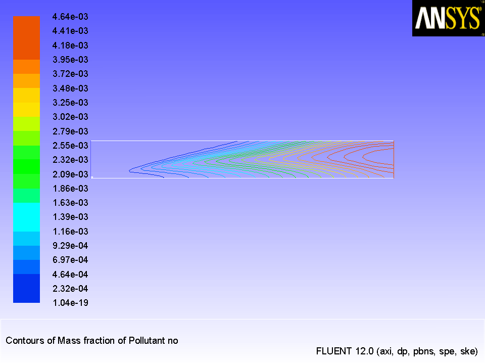
Review the solution by displaying contours of NO mass fraction
(Figure
14.12).
 Graphics and Animations

 Contours
 Set Up...
- (a)
Disable
Filled in the
Options group box.
- (b)
Select
NOx... and
Mass fraction of Pollutant no from the
Contours of drop-down lists.
- (c)
Click
Display and close the
Contours dialog box.
Figure 14.12: Contours of NO Mass Fraction--Prompt and Thermal NOx Formation
 |
-
The peak concentration of NO is located in a region of high temperature where oxygen and nitrogen are available.
- 8.
Calculate the average exit NO mass fraction.
 Reports

 Surface Integrals
 Set Up...
- (a)
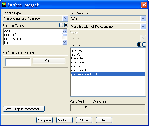
Select
Mass-Weighted Average from the
Report Type drop-down list.
- (b)
Select
NOx... and
Mass fraction of Pollutant no from the
Field Variable drop-down lists.
- (c)
Ensure that
pressure-outlet-9 is selected from the
Surfaces selection list.
- (d)
Click
Compute.
-
The
Mass-Weighted Average field will show that the exit NO mass fraction is approximately 0.0043.
- (e)
Close the
Surface Integrals dialog box.
- 9.
Disable the prompt
NOx mechanism in preparation for solving for thermal
NOx only.
 Models

 NOx
NOx
 Edit...
- (a)
Click the
Formation tab and disable
Prompt NOx.
- (b)
Click
Apply and close the
NOx Model dialog box.
- 10.
Request 50 iterations.
 Run Calculation
-
The solution will converge in less than 10 iterations.
- 11.
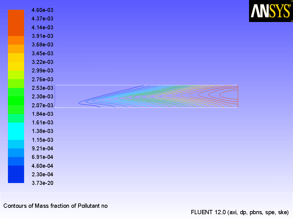
Review the thermal NOx solution by viewing contours of NO mass fraction (Figure
14.13).
 Graphics and Animations

 Contours
 Set Up...
- (a)
Ensure that
NOx... and
Mass fraction of Pollutant no are selected from the
Contours of drop-down list.
- (b)
Click
Display and close the
Contours dialog box.
Figure 14.13: Contours of NO Mass Fraction--Thermal NOx Formation
 |
-
Note that the concentration of NO is slightly lower without the prompt NOx mechanism.
- 12.
Compute the average exit NO mass fraction
with only thermal NOx formation.
 Reports

 Surface Integrals
 Set Up...
-
Hint:
Follow the same procedure you used earlier for the calculation with both thermal and prompt NOx formation.
-
The
Mass-Weighted Average field will show that the exit NO mass fraction with only thermal NOx formation (i.e., with no prompt NOx formation) is approximately 0.0043.
- 13.
Solve for prompt
NOx production only.
 Models

 NOx
NOx
 Edit...
- (a)
Disable
Thermal NOx
in the
Pathways group box.
- (b)
Enable
Prompt NOx.
- (c)
Click
Apply and close the
NOx Model dialog box.
- 14.
Request 50 iterations.
 Run Calculation
-
The solution will converge in less than 10 iterations.
- 15.
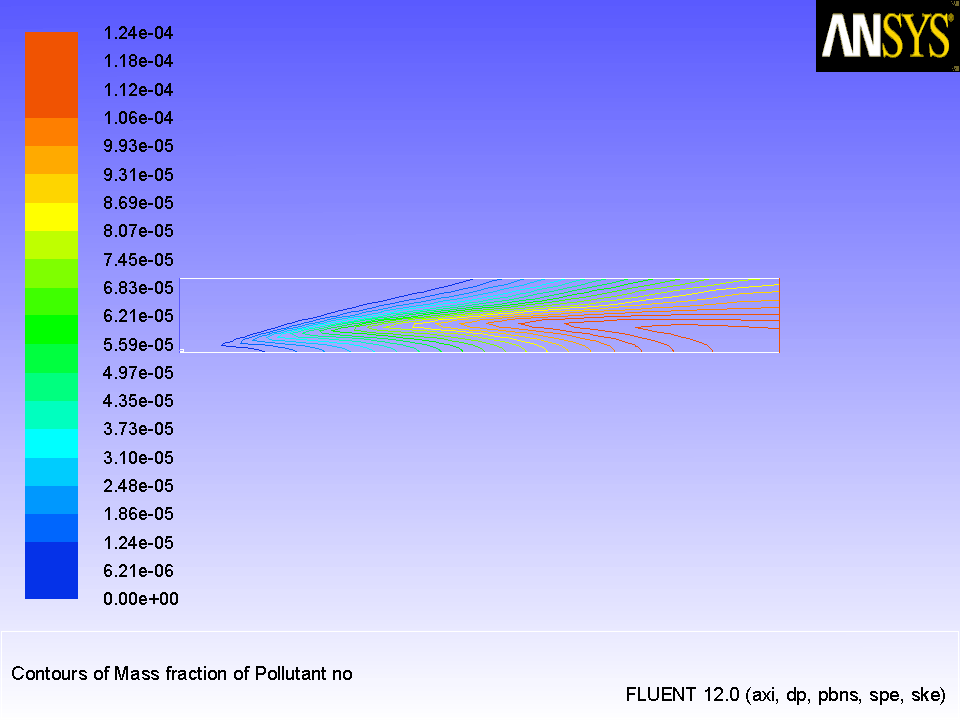
Review the prompt NOx solution by viewing contours of NO mass fraction
(Figure
14.14).
 Graphics and Animations

 Contours
 Set Up...
Figure 14.14: Contours of NO Mass Fraction--Prompt NOx Formation
 |
-
The prompt NOx mechanism is most significant in fuel-rich flames. In this case the flame is lean and prompt NO production is low.
- 16.
Compute the average exit NO mass fraction
with only prompt
NOx formation.
 Reports

 Surface Integrals
 Set Up...
-
Hint:
Follow the same procedure you used earlier for the calculation with both thermal and prompt NOx formation.
-
The
Mass-Weighted Average field will show that the exit NO mass fraction with only prompt NOx formation is approximately 9.74633e-05.
-
Note:
The individual thermal and prompt NO mass fractions do not add up to the levels predicted with the two models combined. This is because reversible reactions are involved. NO produced in one reaction can be destroyed in another reaction.
- 17.
Use a custom field function
to compute NO parts per million (ppm).
-
NO ppm will be computed from the following equation:
 |
(14.14-4) |
Define
 Custom Field Functions...
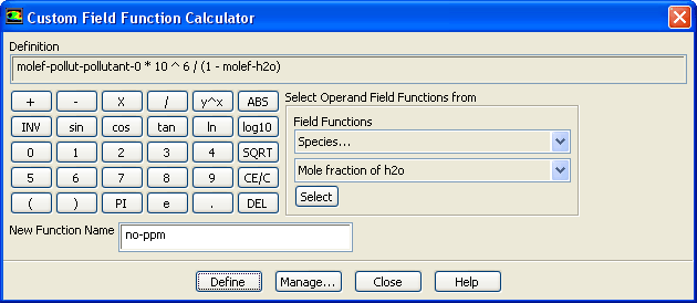
- (a)
Select
NOx... and
Mole fraction of Pollutant no from the
Field Functions drop-down lists, and click the
Select button to enter
molef-pollut-pollutant-0 in the
Definition field.
- (b)
Click the appropriate calculator buttons to enter
*10^6/(1- in the
Definition field, as shown in the previous dialog box.
-
Hint:
If you make a mistake, click the
DEL button on the calculator pad to delete the last item you added to the function definition.
.
- (c)
Select
Species... and
Mole fraction of h2o from the
Field Functions drop-down lists, and click the
Select button to enter
molef-h2o in the
Definition field.
- (d)
Click the
) button to complete the field function.
- (e)
Enter
no-ppm for
New Function Name.
- (f)
Click
Define to add the new field function to the variable list and close the
Custom Field Function Calculator dialog box.
- 18.
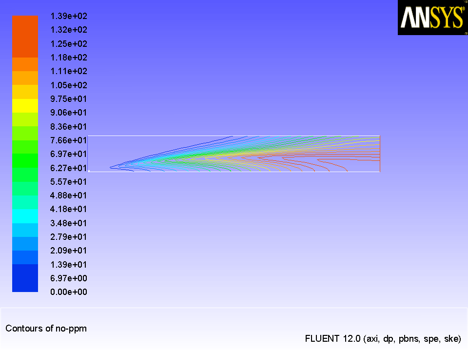
Display contours of NO ppm (Figure
14.15).
 Graphics and Animations

 Contours
 Set Up...
- (a)
Select
Custom Field Functions... and
no-ppm from the
Contours of drop-down lists.
-
Scroll up the list to find
Custom Field Functions....
- (b)
Click
Display and close the
Contours dialog box.
Figure 14.15: Contours of NO ppm--Prompt NOx Formation
 |
-
The contours closely resemble the mass fraction contours (Figure
14.14), as expected.
![[ANSYS, Inc. Logo]](fluentlogo.gif)