- 1.
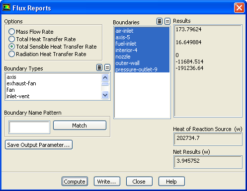
Report the total sensible heat flux.
 Reports

 Fluxes
 Set Up...
- (a)
Select
Total Sensible Heat Transfer Rate in the
Options list.
- (b)
Select all the boundaries from the
Boundaries selection list.
- (c)
Click
Compute and close the
Flux Reports dialog box.
-
Note:
The energy balance is good. The net result is small compared to the heat reaction.
- 2.
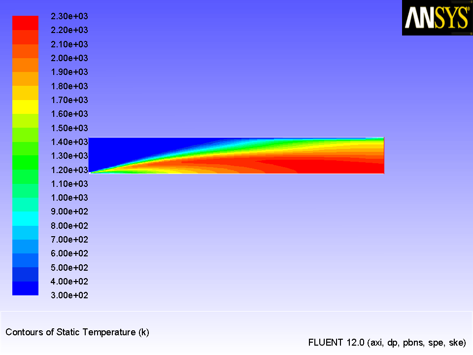
Display filled contours of temperature (Figure
14.4).
 Graphics and Animations

 Contours
 Set Up...
- (a)
Ensure that
Filled is enabled in the
Options group box.
- (b)
Ensure that
Temperature... and
Static Temperature are selected in the
Contours of drop-down lists.
- (c)
Click
Display.
Figure 14.4: Contours of Temperature--Variable

 |
-
The peak temperature has dropped to approximately 2300
 as a result of the temperature and composition-dependent specific heat.
- 3.
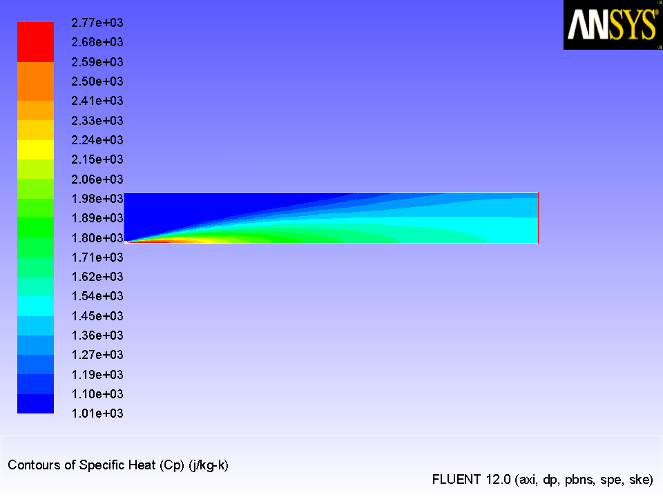
Display filled contours of specific heat (Figure
14.5).
 Graphics and Animations

 Contours
 Set Up...
-
The contours of the mixture specific heat will show the variation of the specific heat within the domain.
- (a)
Select
Properties... and
Specific Heat (Cp) from the
Contours of drop-down lists.
- (b)
Click
Display and close the
Contours dialog box.
-
The mixture specific heat is largest where the CH
 is concentrated, near the fuel inlet, and where the temperature and combustion product concentrations are large. The increase in heat capacity, relative to the constant value used before, substantially lowers the peak flame temperature.
Figure 14.5: Contours of Specific Heat
 |
- 4.
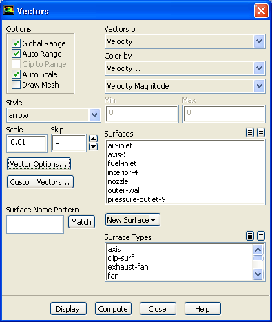
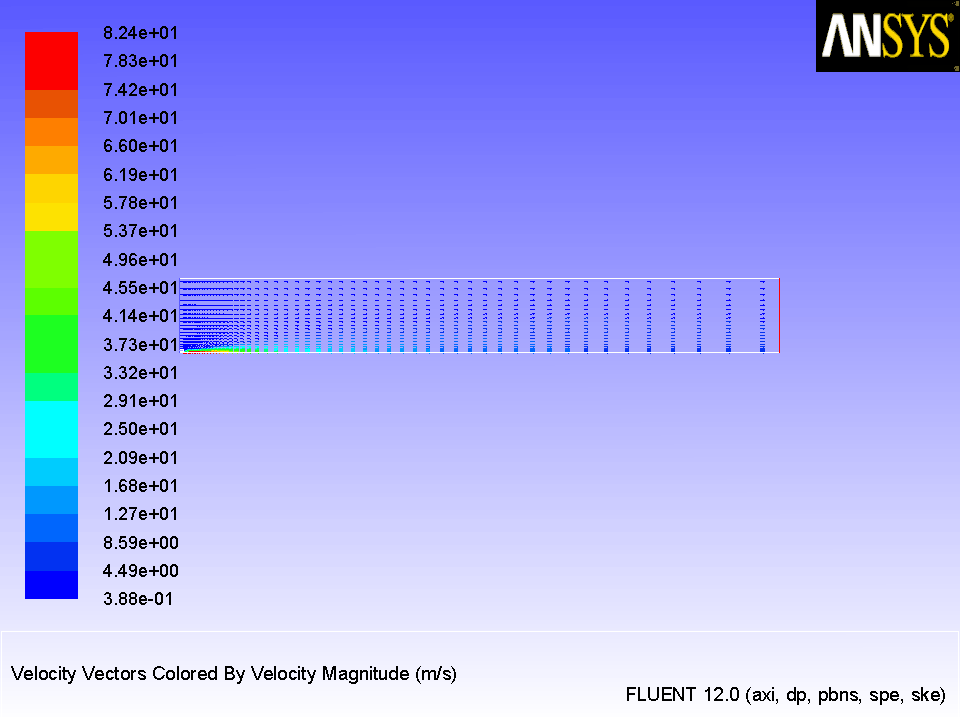
Display velocity vectors (Figure
14.6).
 Graphics and Animations

 Vectors
 Set Up...
- (a)
Enter
0.01 for
Scale.
- (b)
Click the
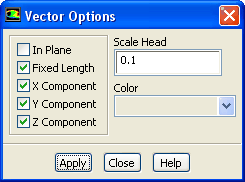
Vector Options... button to open the
Vector Options dialog box.
- i.
Enable
Fixed Length.
-
The fixed length option is useful when the vector magnitude varies dramatically. With fixed length vectors, the velocity magnitude is described only by color instead of by both vector length and color.
- ii.
Click
Apply and close the
Vector Options dialog box.
- (c)
Click
Display and close the
Vectors dialog box.
Figure 14.6: Velocity Vectors--Variable

 |
- 5.
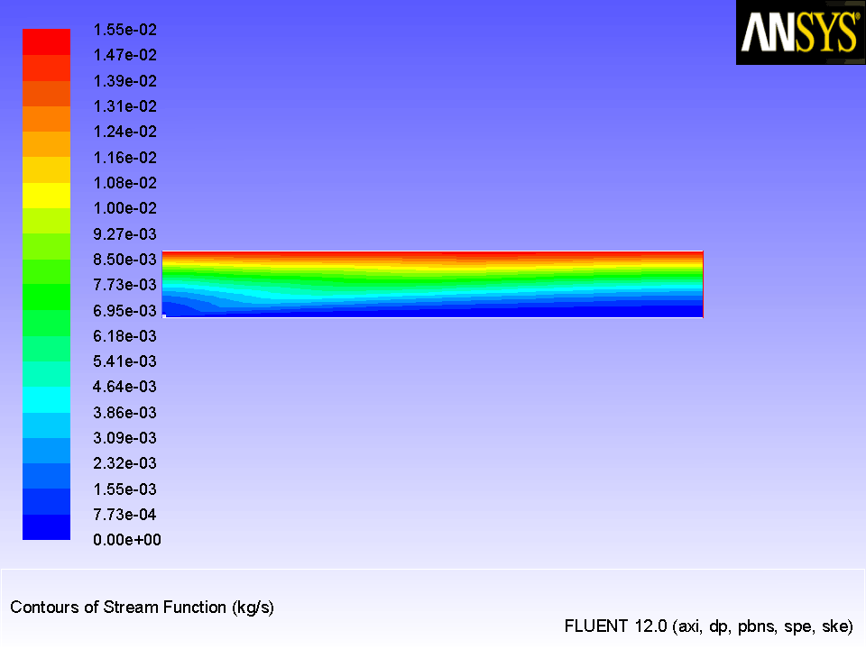
Display filled contours of stream function (Figure
14.7).
 Graphics and Animations

 Contours
 Set Up...
- (a)
Select
Velocity... and
Stream Function from the
Contours of drop-down lists.
- (b)
Click
Display.
Figure 14.7: Contours of Stream Function--Variable

 |
-
The entrainment of air into the high-velocity methane jet is clearly visible in the streamline display.
- 6.
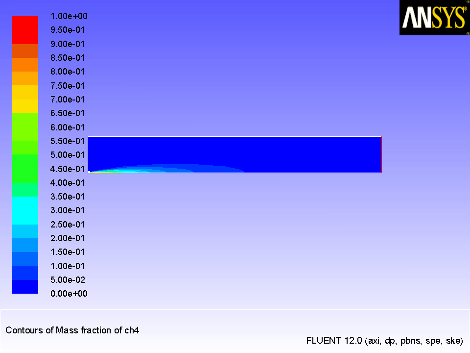
Display filled contours of mass fraction
for CH
 (Figure
14.8).
(Figure
14.8).
 Graphics and Animations

 Contours
 Set Up...
- (a)
Select
Species... and
Mass fraction of ch4 from the
Contours of drop-down lists.
- (b)
Click
Display.
Figure 14.8: Contours of CH
 Mass Fraction
 |
- 7.
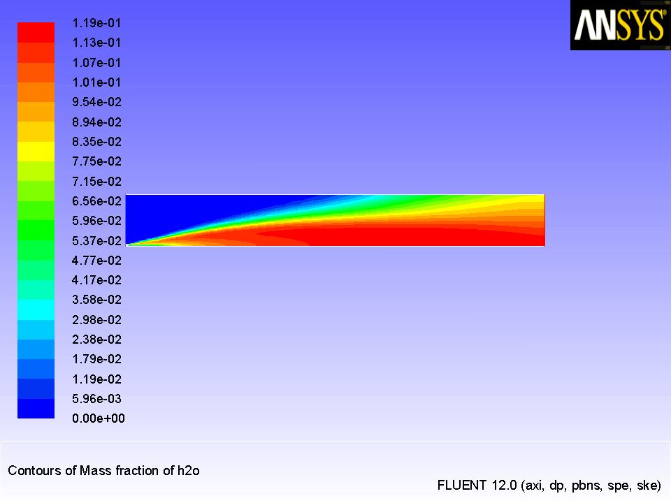
In a similar manner, display the contours of mass fraction for the remaining species O
 , CO
, CO
 , and H
 O (Figures
14.9,
14.10, and
14.11). Close the
Contours dialog box when all of the species have been displayed.
O (Figures
14.9,
14.10, and
14.11). Close the
Contours dialog box when all of the species have been displayed.
Figure 14.9: Contours of O
 Mass Fraction
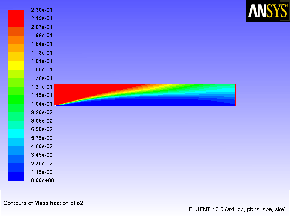 |
Figure 14.10: Contours of CO
 Mass Fraction
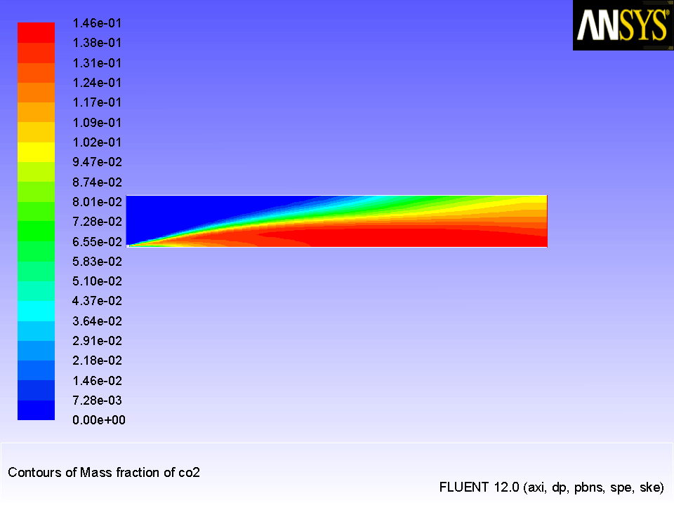 |
Figure 14.11: Contours of H
 O Mass Fraction
 |
- 8.
Determine the average exit temperature.
 Reports

 Surface Integrals
 Set Up...
- (a)
Select
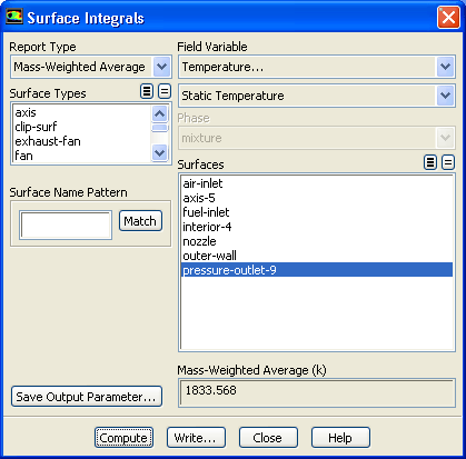
Mass-Weighted Average from the
Report Type drop-down list.
- (b)
Select
Temperature... and
Static Temperature from the
Field Variable drop-down lists.
-
The mass-averaged temperature will be computed as:
 |
(14.13-2) |
- (c)
Select
pressure-outlet-9 from the
Surfaces selection list, so that the integration is performed over this surface.
- (d)
Click
Compute.
-
The
Mass-Weighted Average field will show that the exit temperature is approximately 1834
 .
.
- 9.
Determine the average exit velocity.
 Reports

 Surface Integrals
 Set Up...
- (a)
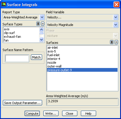
Select
Area-Weighted Average from the
Report Type drop-down list.
- (b)
Select
Velocity... and
Velocity Magnitude from the
Field Variable drop-down lists.
-
The area-weighted velocity-magnitude average will be computed as:
 |
(14.13-3) |
- (c)
Click
Compute.
-
The
Area-Weighted Average field will show that the exit velocity is approximately 3.29
 .
.
- (d)
Close the
Surface Integrals dialog box.
![[ANSYS, Inc. Logo]](fluentlogo.gif)