Step 11: Postprocessing for the Eulerian Model

Graphics and Animations

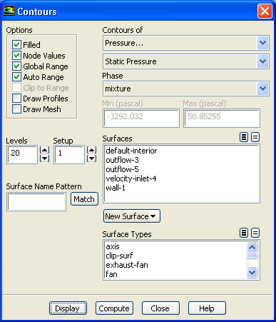
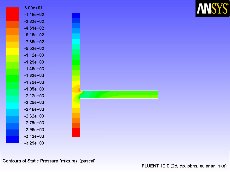
1.   Display the static pressure field in the tee for the mixture (Figure  20.6).

Graphics and Animations Contours Set Up...

(a)   Select Pressure... from the Contours of drop-down list.

  By default, Dynamic Pressure will be displayed in the lower Contours of drop-down list. This will automatically change to Static Pressure after you select the appropriate phase in the next step.

(b)   Select mixture from the Phase drop-down list.

  The lower Contours of drop-down list will now display Static Pressure.

(c)   Click Display.

Figure 20.6: Contours of Static Pressure

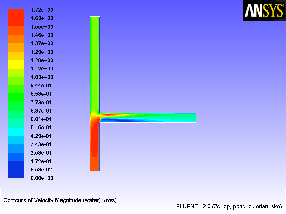
2.   Display contours of velocity magnitude for water (Figure  20.7).

Graphics and Animations Contours Set Up...

(a)   Select Velocity... and Velocity Magnitude from the Contours of drop-down lists.

(b)   Retain the selection of water from the Phase drop-down list.

  Since the Eulerian model solves individual momentum equations for each phase, you can choose the phase for which solution data is plotted.

(c)   Click Display.

Figure 20.7: Contours of Water Velocity Magnitude

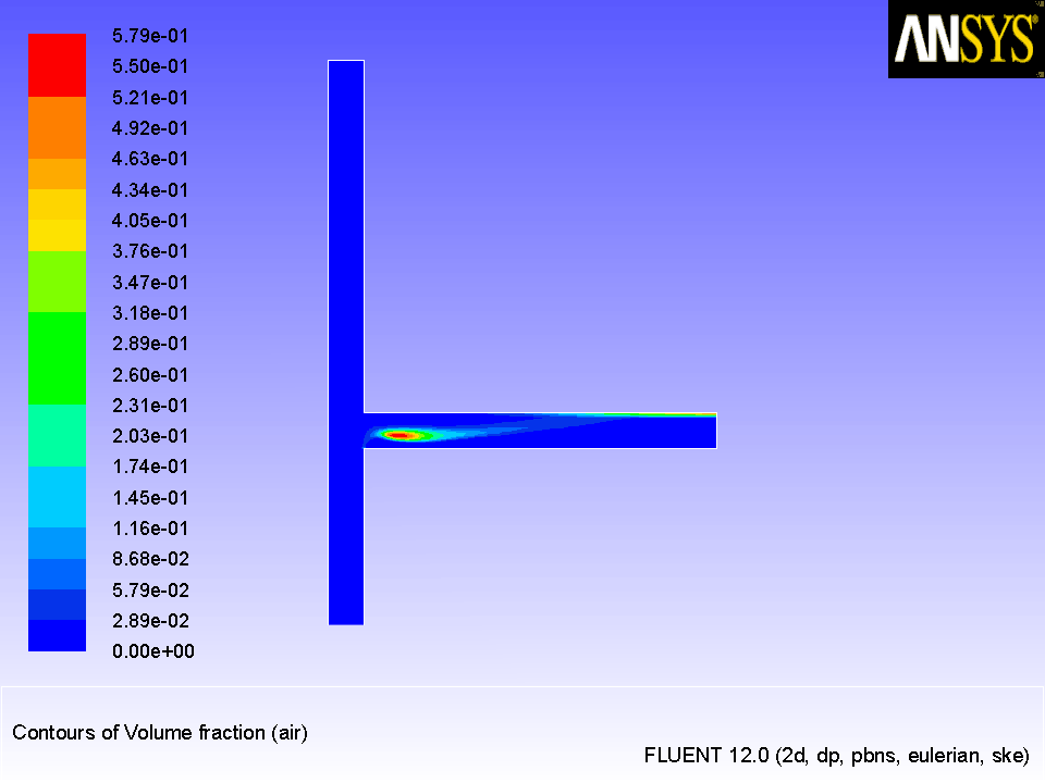
3.   Display the volume fraction of air (Figure  20.8).

Graphics and Animations Contours Set Up...

(a)   Select Phases... and Volume fraction from the Contours of drop-down lists.

(b)   Select air from the Phase drop-down list.

(c)   Click Display and close the Contours dialog box.

Figure 20.8: Contours of Air Volume Fraction