Step 8: Solution

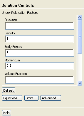
1.   Set the under-relaxation factors.

Solution Controls

(a)   Enter 0.5 for Pressure, 0.2 for Momentum, and 0.8 for Turbulent Viscosity.

Hint:   Scroll down in the Under-Relaxation Factors group box to locate Turbulent Viscosity.

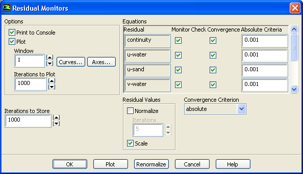
2.   Enable the plotting of residuals during the calculation.

Monitors Residuals Edit...

(a)   Ensure that the Plot is enabled in the Options group box.

(b)   Click OK to close the Residual Monitors dialog box.

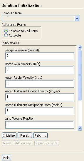
3.   Initialize the solution using the default initial values.

Solution Initialization

(a)   Retain the default initial values and click Initialize.

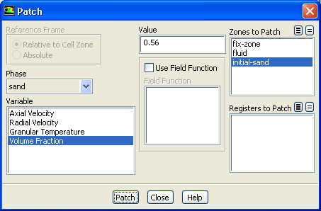
4.   Patch the initial sand bed configuration.

Solution Initialization Patch...

(a)   Select sand from the Phase drop-down list.

(b)   Select Volume Fraction from the Variable selection list.

(c)   Enter 0.56 for Value.

(d)   Select initial-sand from the Zones to Patch selection list.

(e)   Click Patch and close the Patch dialog box.

5.   Save the initial case and data files ( mixtank.cas.gz and mixtank.dat.gz).

File $\rightarrow$ Write $\rightarrow$ Case & Data...

  The problem statement is now complete. As a precaution, you should review the impeller velocity fixes and sand bed patch after running the calculation for a single time step. Since you are using a UDF for the velocity profiles, perform one time step in order for the profiles to be calculated and available for viewing.

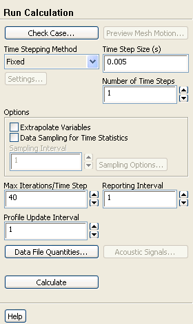
6.   Set the time stepping parameters and run the calculation for 0.005 seconds.

Run Calculation

(a)   Enter 0.005 for Time Step Size.

(b)   Enter 1 for Number of Time Steps.

(c)   Enter 40 for Max Iterations/Time Step.

(d)   Click Calculate.

7.   Examine the initial velocities and sand volume fraction.

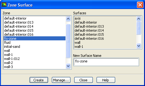
  In order to display the initial fixed velocities in the fluid zone ( fix-zone), you need to create a surface for this zone.

(a)   Create a surface for fix-zone.

Surface $\rightarrow$ Zone...

i.   Select fix-zone from the Zone selection list and click Create.

  The default name is the same as the zone name. ANSYS FLUENT will automatically assign the default name to the new surface when it is created. The new surface will be added to the Surfaces selection list in the Zone Surface dialog box.

ii.   Close the Zone Surface dialog box.

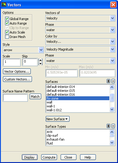
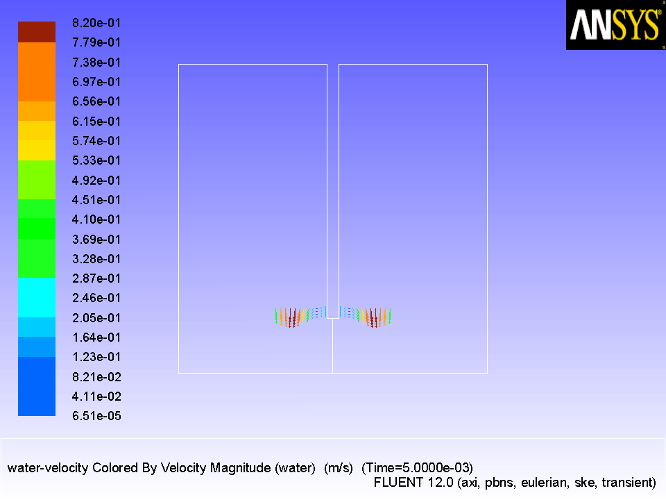
(b)   Display the initial impeller velocities for water (Figure  21.6).

Graphics and Animations Vectors Set Up...

i.   Retain the selection of Velocity from the Vectors of drop-down list.

ii.   Retain the selection of water from the Phase drop-down list below the Vectors of drop-down list.

iii.   Retain the selection of Velocity... and Velocity Magnitude from the Color by drop-down lists.

iv.   Retain the selection of water from the Phase drop-down list below the Color by drop-down lists.

v.   Select fix-zone from the Surfaces selection list and click Display.

   ANSYS FLUENT will display the water velocity vectors fixes at the impeller location, as shown in Figure  21.6.

Figure 21.6: Initial Impeller Velocities for Water

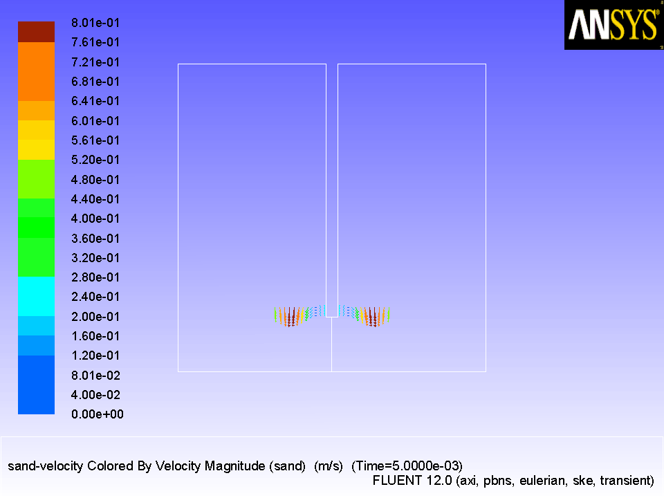
(c)   Display the initial impeller velocities for sand (Figure  21.7).

Graphics and Animations Vectors Set Up...

i.   Select sand from the Phase drop-down lists (below the Vectors of drop-down list and Color by drop-down lists).

ii.   Click Display (Figure  21.7) and close the Vectors dialog box.

Figure 21.7: Initial Impeller Velocities for Sand

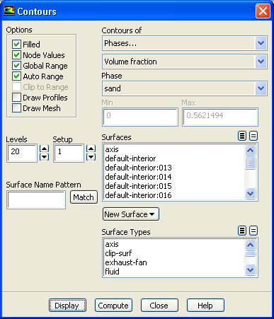
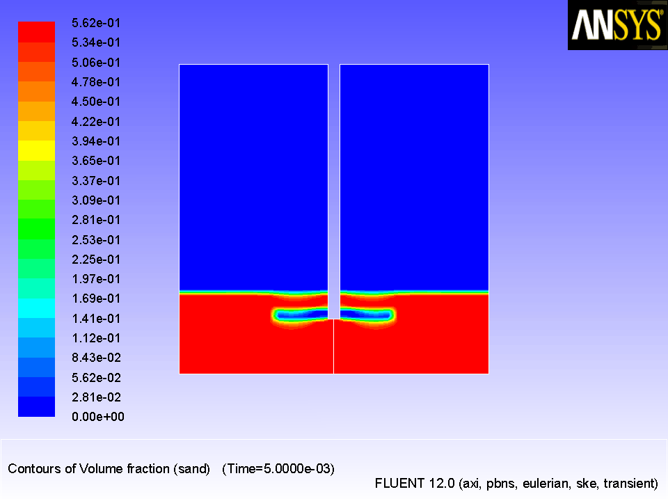
(d)   Display contours of sand volume fraction (Figure  21.8).

Graphics and Animations Contours Set Up...

i.   Enable Filled in the Options group box.

ii.   Select sand from the Phase drop-down list.

iii.   Select Phases... and Volume fraction from the Contours of drop-down lists.

iv.   Click Display and close the Contours dialog box.

   ANSYS FLUENT will display the initial location of the settled sand bed, as shown in Figure  21.8.

Figure 21.8: Initial Settled Sand Bed

8.   Run the calculation for 1 second.

Run Calculation

(a)   Enter 199 for Number of Time Steps.

(b)   Click Calculate.

  After a total of 200 time steps have been computed (1 second of operation), you will review the results before continuing.

9.   Save the case and data files ( mixtank1.cas.gz and mixtank1.dat.gz).

File $\rightarrow$ Write $\rightarrow$ Case & Data...

10.   Examine the results of the calculation after 1 second.

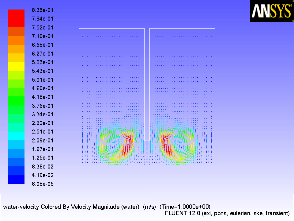
(a)   Display the velocity vectors for water in the whole tank (Figure  21.9).

Graphics and Animations Vectors Set Up...

i.   Select water from the Phase drop-down lists (below the Vectors of drop-down list and Color by drop-down lists).

ii.   Deselect fix-zone from the Surfaces selection list.

iii.   Click Display.

  Figure  21.9 shows the water velocity vectors after 1 second of operation. The circulation is confined to the region near the impeller, and has not yet had time to develop in the upper portions of the tank.

Figure 21.9: Water Velocity Vectors after 1 s

(b)   Display the velocity vectors for the sand (Figure  21.10).

Graphics and Animations Vectors Set Up...

i.   Select sand from the Phase drop-down lists (below the Vectors of drop-down list and Color by drop-down lists).

ii.   Click Display and close the Vectors dialog box.

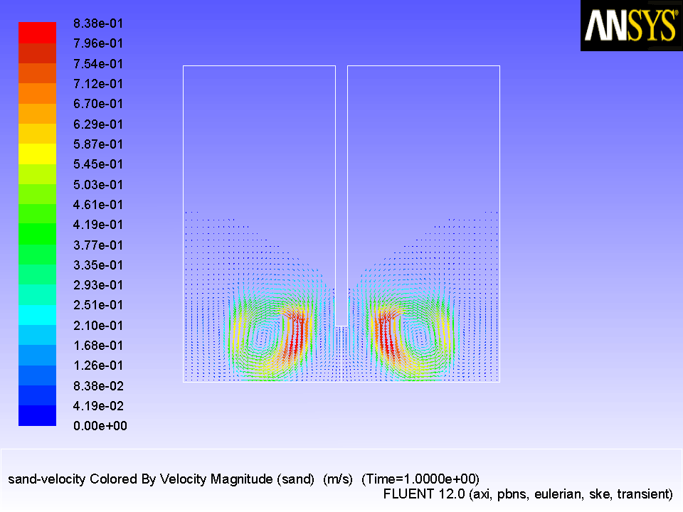
Figure 21.10: Sand Velocity Vectors after 1 s

  Figure  21.10 shows the sand velocity vectors after 1 second of operation. The circulation of sand around the impeller is significant, but note that no sand vectors are plotted in the upper part of the tank, where the sand is not yet present.

(c)   Display contours of sand volume fraction (Figure  21.11).

Graphics and Animations Contours Set Up...

i.   Retain the selection of Phases... and Volume fraction from the Contours of drop-down lists.

ii.   Retain the selection of sand from the Phase drop-down list.

iii.   Click Display and close the Contours dialog box.

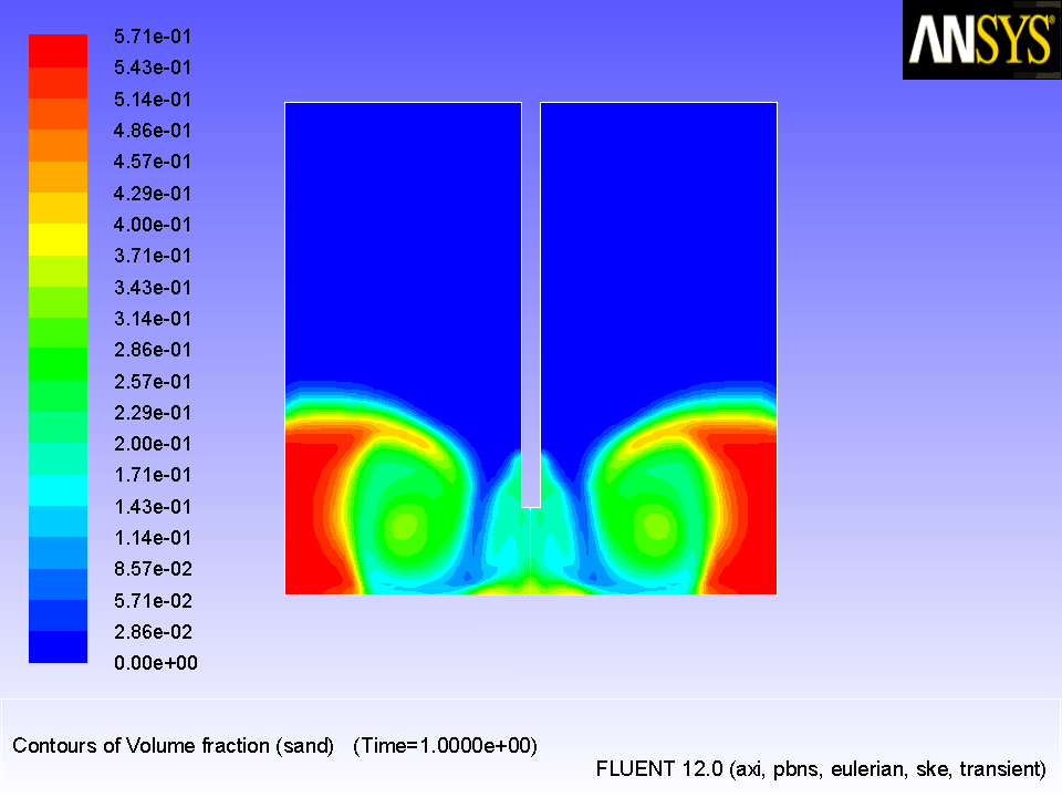
  Notice that the action of the impeller draws clear fluid from above the originally settled bed and mixes it into the sand. To compensate, the sand bed is lifted up slightly. The maximum sand volume fraction has decreased as a result of the mixing of water and sand.

Figure 21.11: Contours of Sand Volume Fraction after 1 s

11.   Continue the calculation for another 19 seconds.

Run Calculation

(a)   Set the Time Step Size to 0.01.

  The initial calculation was performed with a very small time step size to stabilize the solution. After the initial calculation, you can increase the time step to speed up the calculation.

(b)   Enter 1900 for Number of Time Steps.

(c)   Click Calculate.

  The transient calculation will continue upto 20 seconds.

12.   Save the case and data files ( mixtank20.cas.gz and mixtank20.dat.gz).

File $\rightarrow$ Write $\rightarrow$ Case & Data...