Step 8: Solution: Transient Flow and Heat Transfer

  In this step, you will turn on time dependence and include the flow and swirl velocity equations in the calculation. You will then solve the transient problem using the steady conduction solution as the initial condition.

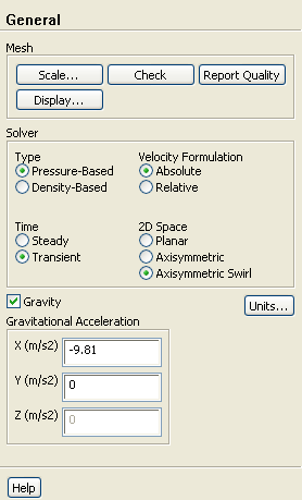
1.   Enable a time-dependent solution.

General

(a)   Select Transient from the Time list.

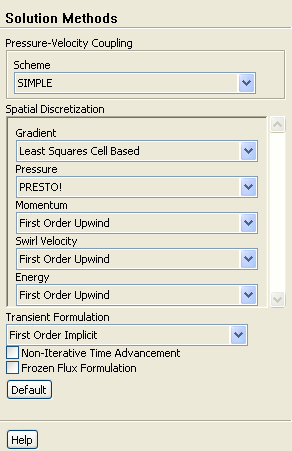
2.   Set the solution parameters.

Solution Methods

(a)   Retain the default selection of First Order Implicit from the Transient Formulation drop-down list.

(b)   Ensure that PRESTO! is selected from the Pressure drop-down list in the Spatial Discretization group box.

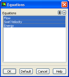
3.   Enable calculations for flow and swirl velocity.

Solution Controls Equations...

(a)   Select Flow and Swirl Velocity and ensure that Energy is selected from the Equations selection list.

  Now all three items in the Equations selection list will be selected.

(b)   Click OK to close the Equations dialog box.

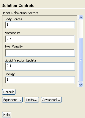
4.   Set the Under-Relaxation Factors.

Solution Controls

(a)   Enter 0.1 for Liquid Fraction Update.

(b)   Retain the default values for other Under-Relaxation Factors.

5.   Save the initial case and data files ( solid01.cas.gz and solid01.dat.gz).

File $\rightarrow$ Write $\rightarrow$ Case & Data...

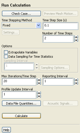
6.   Run the calculation for 2 time steps.

Run Calculation

(a)   Enter 0.1 ${\rm s}$ for Time Step Size.

(b)   Set the Number of Time Steps to 2.

(c)   Retain the default value of 20 for Max Iterations/Time Step.

(d)   Click Calculate.

7.   Display filled contours of the temperature after 0.2 seconds.

Graphics and Animations Contours Set Up...

(a)   Make sure that Temperature... and Static Temperature are selected from the Contours of drop-down lists.

(b)   Click Display (See Figure  22.5).

Figure 22.5: Contours of Temperature at $t$ = 0.2 ${\rm s}$

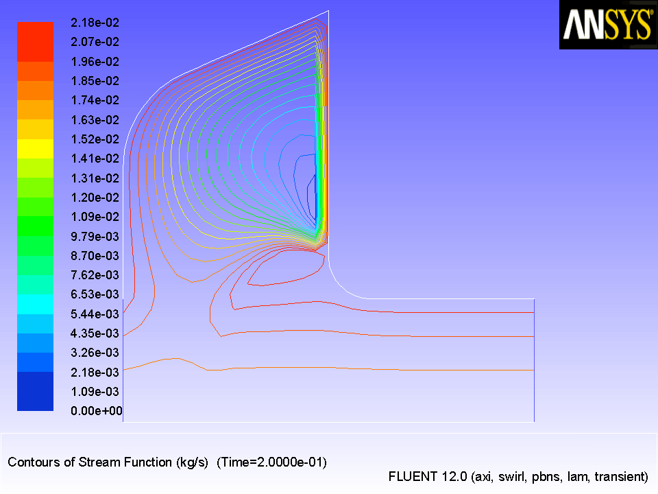
8.   Display contours of stream function (Figure  22.6).

Graphics and Animations Contours Set Up...

(a)   Disable Filled in the Options group box.

(b)   Select Velocity... and Stream Function from the Contours of drop-down lists.

(c)   Click Display.

Figure 22.6: Contours of Stream Function at $t$ = 0.2 ${\rm s}$

  As shown in Figure  22.6, the liquid is beginning to circulate in a large eddy, driven by natural convection and Marangoni convection on the free surface.

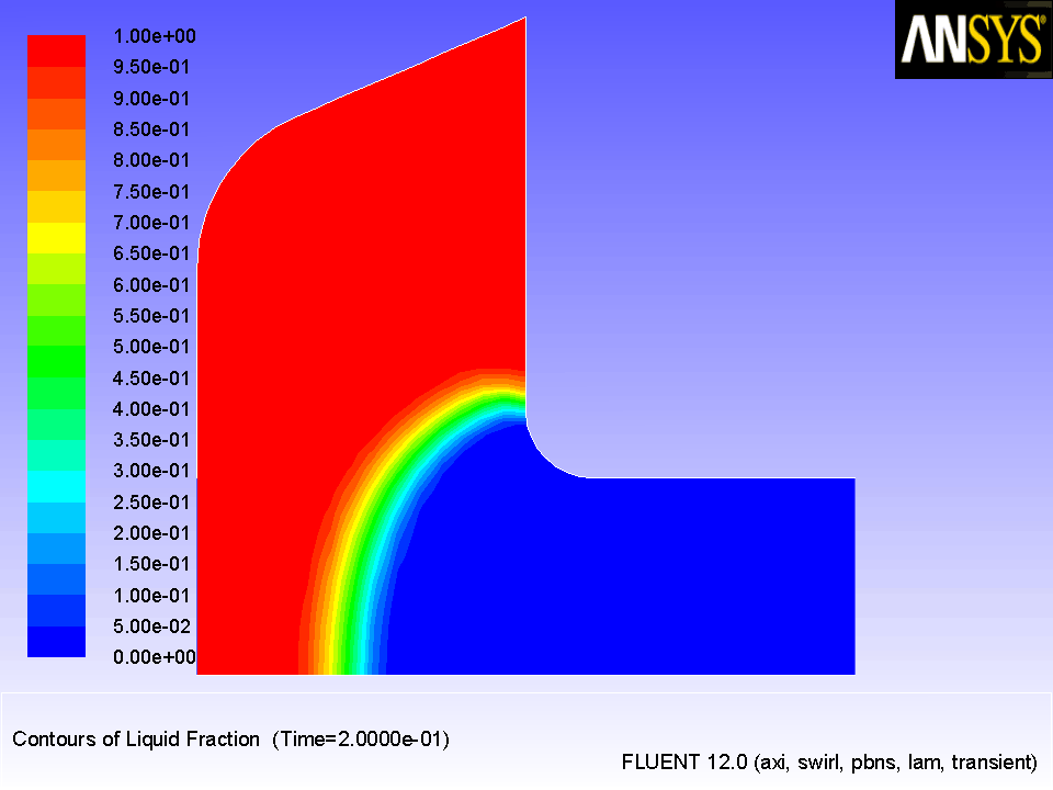
9.   Display contours of liquid fraction (Figure  22.7).

Graphics and Animations Contours Set Up...

(a)   Enable Filled in the Options group box.

(b)   Select Solidification/Melting... and Liquid Fraction from the Contours of drop-down lists.

(c)   Click Display and close the Contours dialog box.

Figure 22.7: Contours of Liquid Fraction at $t$ = 0.2 ${\rm s}$

  The liquid fraction contours show the current position of the melt front. Note that in Figure  22.7, the mushy zone divides the liquid and solid regions roughly in half.

10.   Continue the calculation for 48 additional time steps.

Run Calculation

(a)   Enter 48 for Number of Time Steps.

(b)   Click Calculate.

  After a total of 50 time steps have been completed, the elapsed time will be 5 seconds.

11.   Display filled contours of the temperature after 5 seconds (Figure  22.8).

Graphics and Animations Contours Set Up...

Figure 22.8: Contours of Temperature at $t$ = 5 ${\rm s}$

(a)   Ensure that Filled is enabled in the Options group box.

(b)   Select Temperature... and Static Temperature from the Contours of drop-down lists.

(c)   Click Display.

  As shown in Figure  22.8, the temperature contours are fairly uniform through the melt front and solid material. The distortion of the temperature field due to the recirculating liquid is also clearly evident.

In a continuous casting process, it is important to pull out the solidified material at the proper time. If the material is pulled out too soon, it will not have solidified (i.e., it will still be in a mushy state). If it is pulled out too late, it solidifies in the casting pool and cannot be pulled out in the required shape. The optimal rate of pull can be determined from the contours of liquidus temperature and solidus temperature.

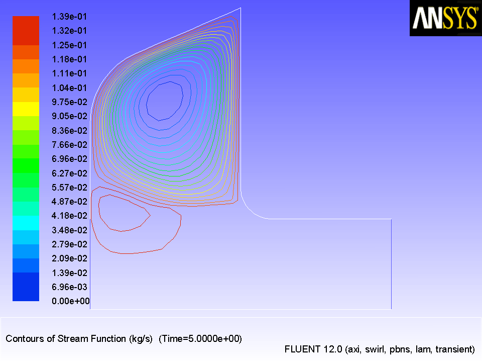
12.   Display contours of stream function (Figure  22.9).

Graphics and Animations Contours Set Up...

(a)   Disable Filled in the Options group box.

(b)   Select Velocity... and Stream Function from the Contours of drop-down lists.

(c)   Click Display.

  As shown in Figure  22.9, the flow has developed more fully by 5 seconds, as compared with Figure  22.6 after 0.2 seconds. The main eddy, driven by natural convection and Marangoni stress, dominates the flow.

  To examine the position of the melt front and the extent of the mushy zone, you will plot the contours of liquid fraction.

Figure 22.9: Contours of Stream Function at $t$ = 5 ${\rm s}$

13.   Display filled contours of liquid fraction (Figure  22.10).

Graphics and Animations Contours Set Up...

(a)   Enable Filled in the Options group box.

(b)   Select Solidification/Melting... and Liquid Fraction from the Contours of drop-down lists.

(c)   Click Display and close the Contours dialog box.

  The introduction of liquid material at the left of the domain is balanced by the pulling of the solidified material from the right. After 5 seconds, the equilibrium position of the melt front is beginning to be established (Figure  22.10).

Figure 22.10: Contours of Liquid Fraction at $t$ = 5 ${\rm s}$

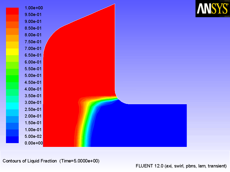14.   Save the case and data files for the solution at 5 seconds ( solid5.cas.gz and solid5.dat.gz).

File $\rightarrow$ Write $\rightarrow$ Case & Data...