Step 7: Solution: Steady Conduction

  In this step, you will specify the discretization schemes to be used and temporarily disable the calculation of the flow and swirl velocity equations, so that only conduction is calculated. This steady-state solution will be used as the initial condition for the time-dependent fluid flow and heat transfer calculation.

1.   Set the solution parameters.

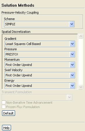
Solution Methods

(a)   Retain the default selection of SIMPLE from the Pressure-Velocity Coupling drop-down list.

(b)   Select PRESTO! from the Pressure drop-down list in the Spatial Discretization group box.

  The PRESTO! scheme is well suited for rotating flows with steep pressure gradients.

(c)   Retain the default selection of First Order Upwind from the Momentum, Swirl Velocity, and Energy drop-down lists.

2.   Enable the calculation for energy.

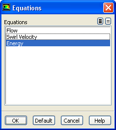
Solution Controls Equations...

(a)   Deselect Flow and Swirl Velocity from the Equations selection list to disable the calculation of flow and swirl velocity equations.

(b)   Click OK to close the Equations dialog box.

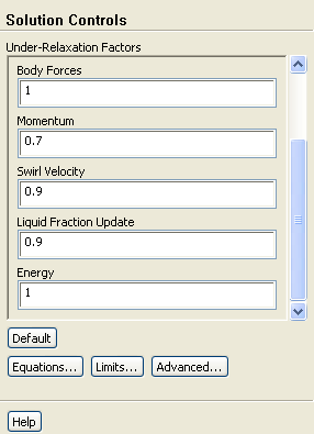
3.   Set the Under-Relaxation Factors.

Solution Controls

(a)   Retain the default values.

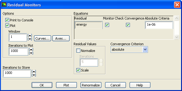
4.   Enable the plotting of residuals during the calculation.

Monitors Residuals Edit...

(a)   Make sure Plot is enabled in the Options group box.

(b)   Click OK to close the Residual Monitors dialog box.

5.   Initialize the solution.

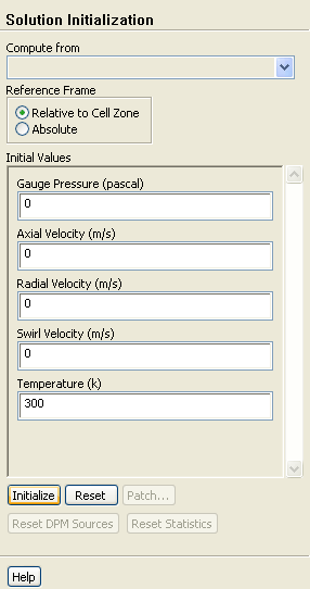
Solution Initialization

(a)   Retain the default value of 0 for Gauge Pressure, Axial Velocity, Radial Velocity, and Swirl Velocity.

  Since you are solving only the steady conduction problem, the initial values for the pressure and velocities will not be used.

(b)   Retain the default value of 300 ${\rm K}$ for Temperature.

(c)   Click Initialize.

6.   Define a custom field function for the swirl pull velocity.

Define $\rightarrow$ Custom Field Functions...

  In this step, you will define a field function to be used to patch a variable value for the swirl pull velocity in the next step. The swirl pull velocity is equal to $\Omega r$, where $\Omega$ is the angular velocity and $r$ is the radial coordinate. Since $\Omega$ = 1 rad/s, you can simplify the equation to simply $r$. In this example, the value of $\Omega$ is included for demonstration purposes.

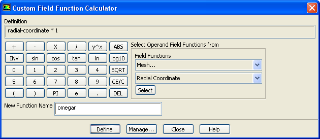
(a)   Select Mesh... and Radial Coordinate from the Field Functions drop-down lists.

(b)   Click the Select button to add radial-coordinate in the Definition field.

  If you make a mistake, click the DEL button on the calculator pad to delete the last item you added to the function definition.

(c)   Click the $\times$ button on the calculator pad.

(d)   Click the 1 button.

(e)   Enter omegar for New Function Name.

(f)   Click Define.

Note:   To check the function definition, you can click Manage... to open the Field Function Definitions dialog box. Then select omegar from the Field Functions selection list to view the function definition.

(g)   Close the Custom Field Function Calculator dialog box.

7.   Patch the pull velocities.

Solution Initialization Patch...

  As noted earlier, you will patch values for the pull velocities, rather than having ANSYS FLUENT compute them. Since the radial pull velocity is zero, you will patch just the axial and swirl pull velocities.

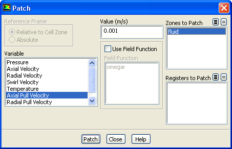
(a)   Select Axial Pull Velocity from the Variable selection list.

(b)   Enter 0.001 ${\rm m/s}$ for Value.

(c)   Select fluid from the Zones to Patch selection list.

(d)   Click Patch.

  You have just patched the axial pull velocity. Next you will patch the swirl pull velocity.

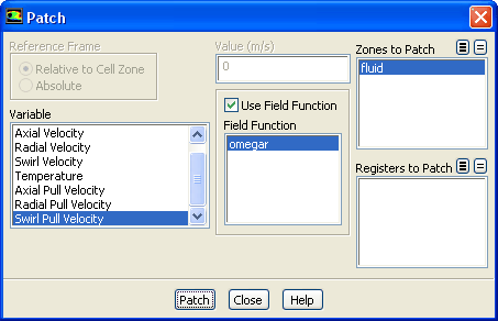
(e)   Select Swirl Pull Velocity from the Variable selection list.

  Scroll down the list to find Swirl Pull Velocity.

(f)   Enable the Use Field Function option.

(g)   Select omegar from the Field Function selection list.

(h)   Make sure that fluid is selected from the Zones to Patch selection list.

(i)   Click Patch and close the Patch dialog box.

8.   Save the initial case and data files ( solid0.cas.gz and solid0.dat.gz).

File $\rightarrow$ Write $\rightarrow$ Case & Data...

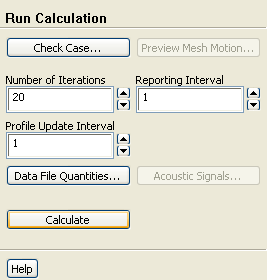
9.   Start the calculation by requesting 20 iterations.

Run Calculation

(a)   Enter 20 for Number of Iterations.

(b)   Click Calculate.

  The solution will converge in approximately 11 iterations.

10.   Display filled contours of temperature (Figure  22.3).

Graphics and Animations Contours Set Up...

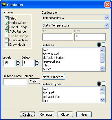
(a)   Enable the Filled option.

(b)   Select Temperature... and Static Temperature from the Contours of drop-down lists.

(c)   Click Display (Figure  22.3).

Figure 22.3: Contours of Temperature for the Steady Conduction Solution

11.   Display filled contours of temperature to determine the thickness of mushy zone.

Graphics and Animations Contours Set Up...

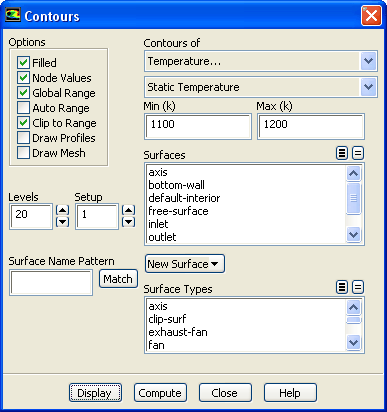
(a)   Disable Auto Range in the Options group box.

  The Clip to Range option will automatically be enabled.

(b)   Enter 1100 for Min and 1200 for Max.

(c)   Click Display (See Figure  22.4) and close the Contours dialog box.

Figure 22.4: Contours of Temperature (Mushy Zone) for the Steady Conduction Solution

12.   Save the case and data files for the steady conduction solution ( solid.cas.gz and solid.dat.gz).

File $\rightarrow$ Write $\rightarrow$ Case & Data...