![[ANSYS, Inc. Logo]](fluentlogo.gif)


|
|
|
The P-1 radiation model is the simplest case of the more general P-N model, which is based on the expansion of the radiation intensity
 into an orthogonal series of spherical harmonics [
52,
315]. This section provides details about the equations used in the P-1 model. For information about setting up the model, see
this section in the separate
User's Guide.
into an orthogonal series of spherical harmonics [
52,
315]. This section provides details about the equations used in the P-1 model. For information about setting up the model, see
this section in the separate
User's Guide.
The P-1 Model Equations
As mentioned above, the P-1 radiation model is the simplest case of the P-N model. If only four terms in the series are used, the following equation is obtained for the radiation flux
 :
:
where
 is the absorption coefficient,
 is the scattering coefficient,
 is the incident radiation, and
 is the linear-anisotropic phase function coefficient, described below. After introducing the parameter
Equation 5.3-2 simplifies to
The transport equation for
 is
is
where
 is the refractive index of the medium,
 is the Stefan-Boltzmann constant and
 is a user-defined radiation source.
ANSYS FLUENT solves this equation to determine the local radiation intensity when the P-1 model is active.
is a user-defined radiation source.
ANSYS FLUENT solves this equation to determine the local radiation intensity when the P-1 model is active.
Combining Equations 5.3-4 and 5.3-5 yields the following equation:
 |
(5.3-6) |
The expression for
 can be directly substituted into the energy equation to account for heat sources (or sinks) due to radiation.
Anisotropic Scattering
Included in the P-1 radiation model is the capability for modeling anisotropic scattering. ANSYS FLUENT models anisotropic scattering by means of a linear-anisotropic scattering phase function:
Here,
 is the unit vector in the direction of scattering, and
 is the unit vector in the direction of the incident radiation.
 is the linear-anisotropic phase function coefficient, which is a property of the fluid.
 ranges from
 to 1. A positive value indicates that more radiant energy is scattered forward than backward, and a negative value means that more radiant energy is scattered backward than forward. A zero value defines isotropic scattering (i.e., scattering that is equally likely in all directions), which is the default in
ANSYS FLUENT. You should modify the default value only if you are certain of the anisotropic scattering behavior of the material in your problem.
to 1. A positive value indicates that more radiant energy is scattered forward than backward, and a negative value means that more radiant energy is scattered backward than forward. A zero value defines isotropic scattering (i.e., scattering that is equally likely in all directions), which is the default in
ANSYS FLUENT. You should modify the default value only if you are certain of the anisotropic scattering behavior of the material in your problem.
Particulate Effects in the P-1 Model
When your ANSYS FLUENT model includes a dispersed second phase of particles, you can include the effect of particles in the P-1 radiation model. Note that when particles are present, ANSYS FLUENT ignores scattering in the gas phase. (That is, Equation 5.3-8 assumes that all scattering is due to particles.)
For a gray, absorbing, emitting, and scattering medium containing absorbing, emitting, and scattering particles, the transport equation for the incident radiation can be written as
where
 is the equivalent emission of the particles,
 is the equivalent absorption coefficient, and
 is the refractive index of the medium. These are defined as follows:
and
In Equations
5.3-9 and
5.3-10,
 ,
,
 , and
, and
 are the emissivity, projected area, and temperature of particle
 . The summation is over
 particles in volume
 . These quantities are computed during particle tracking in
ANSYS FLUENT.
. These quantities are computed during particle tracking in
ANSYS FLUENT.
The projected area
 of particle
 is defined as
 |
(5.3-11) |
where
 is the diameter of the
 th particle.
The quantity
 in Equation
5.3-8 is defined as
in Equation
5.3-8 is defined as
 |
(5.3-12) |
where the equivalent particle scattering factor is defined as
and is computed during particle tracking. In Equation
5.3-13,
 is the scattering factor associated with the
 th particle.
Heat sources (sinks) due to particle radiation are included in the energy equation as follows:
 |
(5.3-14) |
Boundary Condition Treatment for the P-1 Model at Walls
To get the boundary condition for the incident radiation equation, the dot product of the outward normal vector
 and Equation
5.3-4 is computed:
and Equation
5.3-4 is computed:
Thus the flux of the incident radiation,
 , at a wall is
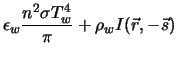
 . The wall radiative heat flux is computed using the following boundary condition:
where
 is the wall reflectivity. The Marshak boundary condition is then used to eliminate the angular dependence [
262]:
is the wall reflectivity. The Marshak boundary condition is then used to eliminate the angular dependence [
262]:
Substituting Equations 5.3-17 and 5.3-18 into Equation 5.3-19 and performing the integrations yields
If it is assumed that the walls are diffuse gray surfaces, then
 , and Equation
5.3-20 becomes
, and Equation
5.3-20 becomes
Equation
5.3-21 is used to compute
 for the energy equation and for the incident radiation equation boundary conditions.
Boundary Condition Treatment for the P-1 Model at Flow Inlets and Exits
The net radiative heat flux at flow inlets and outlets is computed in the same manner as at walls, as described above. ANSYS FLUENT assumes that the emissivity of all flow inlets and outlets is 1.0 (black body absorption) unless you choose to redefine this boundary treatment.
ANSYS FLUENT includes an option that allows you to use different temperatures for radiation and convection at inlets and outlets. This can be useful when the temperature outside the inlet or outlet differs considerably from the temperature in the enclosure. See this section in the separate User's Guide for details.
Previous:
5.3.2 Radiative Transfer Equation