2.3.3 The Quadrature Method of Moments (QMOM)

The quadrature method of moments (QMOM) was first proposed by McGraw [ 21] for modeling aerosol evolution and coagulation problems. Its applications by Marchisio et al. [ 19] have shown that the method requires a relatively small number of scalar equations to track the moments of population with small errors.

The QMOM provides an attractive alternative to the discrete method when aggregation quantities, rather than an exact PSD, are desired. Its advantages are fewer variables (typically only six or eight moments) and a dynamic calculation of the size bins. The disadvantages are that the number of abscissas may not be adequate to describe the PSD and that solving the Product-Difference algorithm may be time consuming.

Numerical Method

The quadrature approximation is based on determining a sequence of polynomials orthogonal to $n(L)$ (i.e., the particle size distribution). If the abscissas of the quadrature approximation are the nodes of the polynomial of order $N$, then the quadrature approximation

is exact if $f(L)$ is a polynomial of order $N$ or smaller [ 5]. In all other cases, the closer $f(L)$ is to a polynomial, the more accurate the approximation.

A direct way to calculate the quadrature approximation is by means of its definition through the moments:

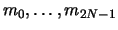The quadrature approximation of order $N$ is defined by its $N$ weights $w_i$ and $N$ abscissas $L_i$ and can be calculated by its first $2N$ moments $m_0,\dots,m_{2N-1}$ by writing the recursive relationship for the polynomials in terms of the moments $m_k$. Once this relationship is written in matrix form, it is easy to show that the roots of the polynomials correspond to the eigenvalues of the Jacobi matrix [ 24]. This procedure is known as the Product-Difference algorithm [ 8]. Once the weights and abscissas are known, the source terms due to coalescence and breakage can be calculated and therefore the transport equations for the moments can be solved.

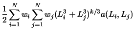
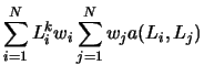
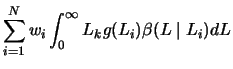
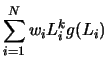
Applying Equations  2.3-31 and 2.3-32, the birth and death terms in Equation  2.3-19 can be rewritten as

$$\overline{B}_{{\rm ag},k} = \frac{1}{2}\sum_{i=1}^{N}w_{i}\sum_{j=1}^{N}w_{j} (L_{i}^{3}+L_{j}^{3})^{k/3}a(L_{i},L_{j})$$ (2.3-33)

$$\overline{D}_{{\rm ag},k} = \sum_{i=1}^{N}L_{i}^{k}w_{i}\sum_{j=1}^{N}w_{j} a(L_{i},L_{j})$$ (2.3-34)

$$\overline{B}_{{\rm br},k} = \sum_{i=1}^{N}w_{i}\int_0^{\infty}L_{k}g(L_{i})\beta(L \mid L_{i})dL$$ (2.3-35)

$$\overline{D}_{{\rm br},k} = \sum_{i=1}^{N}w_{i}L_{i}^{k}g(L_{i})$$ (2.3-36)

Theoretically, there is no limitation on the expression of breakage and aggregation kernels when using QMOM.

The nucleation rate is defined in the same way as for the SMM. The growth rate for QMOM is defined by Equation  2.3-24 and represented as

to allow for a size-dependent growth rate.