Step 6: Initial Solution with Constant Heat Capacity

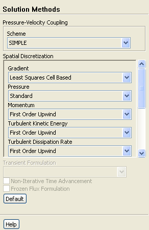
1.   Retain the default solution parameters.

Solution Methods

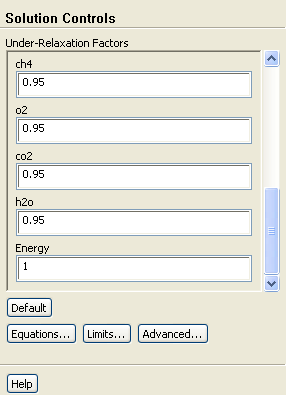
2.   Set the under-relaxation factors for the species.

Solution Controls

  The default under-relaxation parameters in ANSYS FLUENT are set to high values. For a combustion model, it may be necessary to reduce the under-relaxation to stabilize the solution. Some experimentation is typically necessary to establish the optimal under-relaxation. For this tutorial, it is sufficient to reduce the species under-relaxation to 0.95.

(a)   Enter 0.95 for each of the species ( ch4, o2, co2, and h2o) in the Under-Relaxation Factors group box.

  Scroll down the Under-Relaxation Factors group box to find the species.

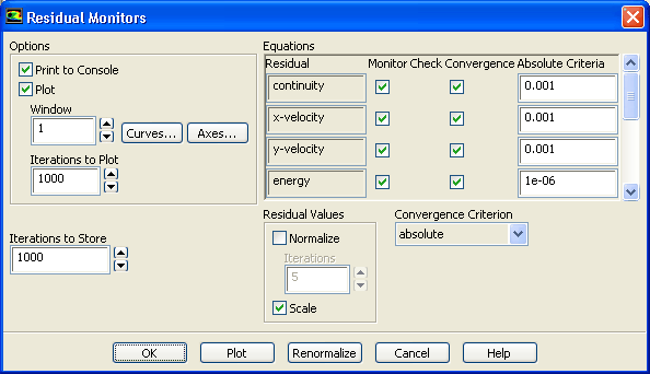
3.   Ensure the plotting of residuals during the calculation.

Monitors Residuals Edit...

(a)   Ensure that Plot is enabled in the Options group box.

(b)   Click OK to close the Residual Monitors dialog box.

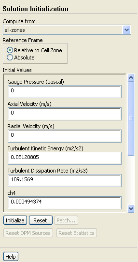
4.   Initialize the field variables.

Solution Initialization

(a)   Select all-zones from the Compute From drop-down list.

(b)   Click Initialize to initialize the variables.

5.   Save the case file ( gascomb1.cas.gz).

File $\rightarrow$ Write $\rightarrow$ Case...

(a)   Enter gascomb1.cas.gz for Case File.

(b)   Ensure that Write Binary Files is enabled to produce a smaller, unformatted binary file.

(c)   Click OK close the Select File dialog box.

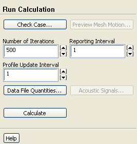
6.   Start the calculation by requesting 500 iterations.

Run Calculation

  The solution will converge in approximately 280 iterations.

7.   Save the case and data files ( gascomb1.cas.gz and gascomb1.dat.gz).

File $\rightarrow$ Write $\rightarrow$ Case & Data...

Note:   If you choose a file name that already exists in the current folder, ANSYS FLUENT will ask you to confirm that the previous file is to be overwritten.

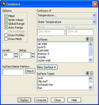
8.   Review the current state of the solution by displaying filled contours of temperature.

Graphics and Animations Contours Set Up...

(a)   Enable Filled in the Options group box.

(b)   Select Temperature... and Static Temperature from the Contours of drop-down lists.

(c)   Click Display (See Figure  14.3) and close the Contours dialog box.

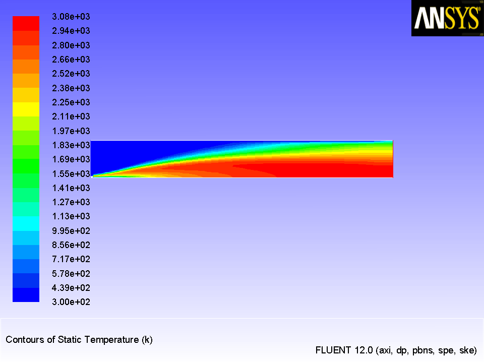
Figure 14.3: Contours of Temperature: Constant $C_p$

  The peak temperature, predicted using a constant heat capacity of 1000  ${\rm J/kg-K}$, is over 3000  ${\rm K}$. This overprediction of the flame temperature can be remedied by a more realistic model for the temperature and composition dependence of the heat capacity, as illustrated in the next step of the tutorial.