Step 3: Models

Models

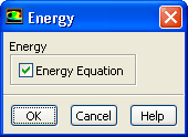
1.   Enable the Energy Equation.

Models Energy Edit...

(a)   Enable Energy Equation.

(b)   Click OK to close the Energy dialog box.

  Since heat transfer occurs in the system considered here, you will have to solve the energy equation.

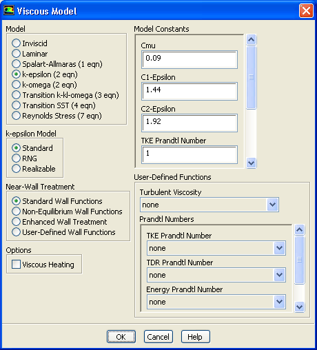
2.   Select the standard k-epsilon turbulence model.

Models Viscous Edit...

(a)   Select k-epsilon (2 eqn) in the Model list.

  For axisymmetric swirling flow, the RNG k-epsilon model can also be used.

(b)   Retain all other default settings.

(c)   Click OK to close the Viscous Model dialog box.

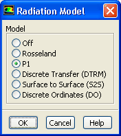
3.   Select the P1 radiation model.

Models Radiation Edit...

(a)   Select P1 in the Model list.

(b)   Click OK to close the Radiation Model dialog box.

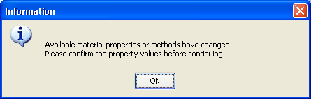
  The ANSYS FLUENT console will list the properties that are required for the model you have enabled. An Information dialog box will open, reminding you to confirm the property values.

(c)   Click OK to close the Information dialog box.

  The DO radiation model produces a more accurate solution than the P1 radiation model but it can be CPU intensive. The P1 model will produce a quick, acceptable solution for this problem.

For details on the different radiation models available in ANSYS FLUENT, see this chapter in the separate User's Guide.

4.   Select the Non-Premixed Combustion model.

Models Species Edit...

(a)   Select Non-Premixed Combustion in the Model list.

  The dialog box will expand to show the related inputs. You will use this dialog box to create the PDF table.

  When you use the non-premixed combustion model, you need to create a PDF table. This table contains information on the thermo-chemistry and its interaction with turbulence. ANSYS FLUENT interpolates the PDF during the solution of the non-premixed combustion model.

(b)   Enable Inlet Diffusion in the PDF Options group box.

  The Inlet Diffusion option enables the mixture fraction to diffuse out of the domain through inlets and outlets.

(c)   Define chemistry models.

i.   Retain the default selection of Equilibrium and Non-Adiabatic.

  In most non-premixed combustion simulations, the Equilibrium chemistry model is recommended. The Steady Flamelets option can model local chemical non-equilibrium due to turbulent strain.

ii.   Retain the default value for Operating Pressure.

iii.   Enter 0.064 for Fuel Stream Rich Flammability Limit.

  For combustion cases, a value larger than 10% - 50% of the stoichiometric mixture fraction can be used for the rich flammability limit of the fuel stream. In this case, the stoichiometric fraction is 0.058, therefore a value that is 10% greater is 0.064.

  The Fuel Stream Rich Flammability Limit allows you to perform a "partial equilibrium'' calculation, suspending equilibrium calculations when the mixture fraction exceeds the specified rich limit. This increases the efficiency of the PDF calculation, allowing you to bypass the complex equilibrium calculations in the fuel-rich region. This is also more physically realistic than the assumption of full equilibrium.

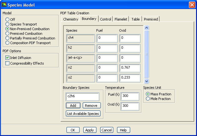
(d)   Click the Boundary tab to add and define the boundary species.

i.   Add c2h6, c3h8, c4h10, and co2.

a.   Enter c2h6 in the Boundary Species text-entry field and click Add.

b.   Similarly, add c3h8, c4h10, and co2.

  All the four species will appear in the table.

ii.   Select Mole Fraction in the Species Unit list.

iii.   Retain the default values for n2 and o2 for Oxid.

  The oxidizer (air) consists of 21% O $_2$ and 79% N $_2$ by volume.

iv.   Specify the fuel composition by entering the following values for Fuel:

  The fuel composition is entered in mole fractions of the species, c2h6, c3h8, c4h10, and co2.

Species	Mole Fraction
ch4	0.965
n2	0.013
c2h6	0.017
c3h8	0.001
c4h10	0.001
co2	0.003

Hint:   Scroll down to see all the species.

Note:   All boundary species with a mass or mole fraction of zero will be ignored.

v.   Enter 315 K for Fuel and Oxid in the Temperature group box.

(e)   Click the Control tab and retain default species to be excluded from the equilibrium calculation.

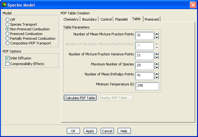
(f)   Click the Table tab to specify the table parameters and calculate the PDF table.

i.   Retain the default values for all the parameters in the Table Parameters group box.

  The maximum number of species determines the number of most preponderant species to consider after the equilibrium calculation is performed.

ii.   Click Calculate PDF Table to compute the non-adiabatic PDF table.

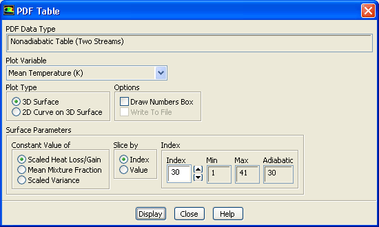
iii.   Click the Display PDF Table... button to open the PDF Table dialog box.

a.   Retain the default parameters and click Display (Figure  15.5).

b.   Close the PDF Table dialog box.

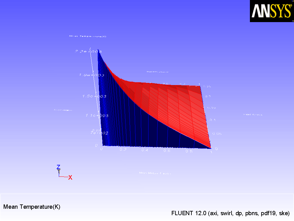
Figure 15.5: Non-Adiabatic Temperature Look-Up Table on the Adiabatic Enthalpy Slice

  The 3D look-up tables are reviewed on a slice-by-slice basis. By default, the slice selected is that corresponding to the adiabatic enthalpy values. You can also select other slices of constant enthalpy for display.

  The maximum and minimum values for mean temperature and the corresponding mean mixture fraction will also be reported in the console. The maximum mean temperature is reported as 2246 K at a mean mixture fraction of 0.058.

(g)   Save the PDF output file ( berl.pdf).

File $\rightarrow$ Write $\rightarrow$ PDF...

i.   Retain berl.pdf for PDF File name.

ii.   Click OK to write the file.

  By default, the file will be saved as formatted (ASCII, or text). To save a binary (unformatted) file, enable the Write Binary Files option in the Select File dialog box.

(h)   Click OK to close the Species Model dialog box.