Step 9: Postprocessing

1.   Create an iso-surface near wall-4.

Surface $\rightarrow$ Iso-Surface...

(a)   Select Mesh and Z-Coordinate from the Surface of Constant drop-down lists.

(b)   Click Compute.

(c)   Enter 0.075438 m for Iso-Values.

(d)   Enter z=0.07 for New Surface Name.

(e)   Click Create and close the Iso-Surface dialog box.

2.   Display contours of temperature on the plane surface created. (Figure  16.6).

Graphics and Animations Contours Set Up...

(a)   Ensure that Filled is enabled in the Options group box.

(b)   Select Temperature... and Static Temperature from the Contours of drop-down lists.

(c)   Deselect wall-4 from the Surfaces selection list.

(d)   Select z=0.07 from the Surfaces selection list.

(e)   Click Display.

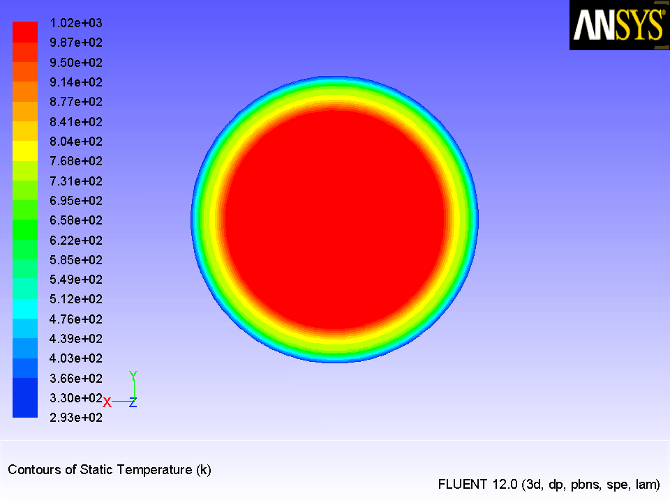
Figure 16.6: Temperature Contours Near wall-4

  Figure  16.6 shows the temperature distribution across a plane just above the rotating disk. You can see that the disk has a temperature of 1023 K.

3.   Display contours of surface deposition rates of ga (Figure  16.7).

Graphics and Animations Contours Set Up...

(a)   Select Species... and Surface Deposition Rate of ga from the Contours of drop-down lists.

(b)   Select wall-4 from the Surfaces selection list.

(c)   Deselect z=0.07 from the Surfaces selection list.

(d)   Click Display.

   You may need to use the left mouse button to rotate the image so that you can see the contours on the top side of wall-4 where the deposition takes place.

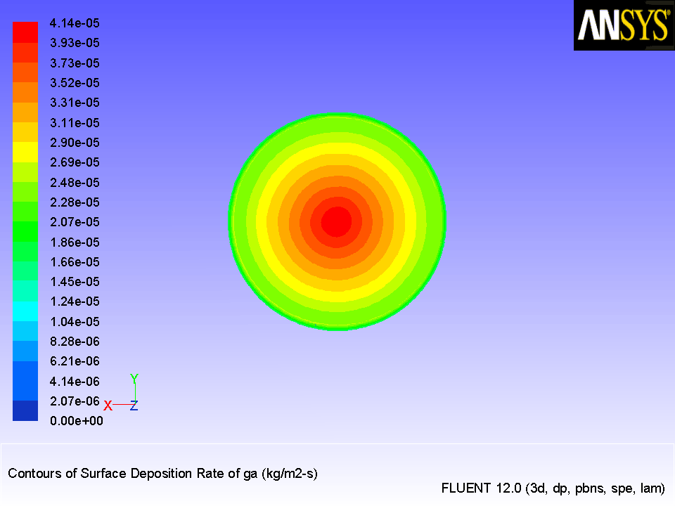
  Figure  16.7 shows the gradient of surface deposition rate of ga. The maximum deposition is seen at the center of the disk.

Figure 16.7: Contours of Surface Deposition Rate of ga

4.   Display contours of surface coverage of ga_s (Figure  16.8).

Graphics and Animations Contours Set Up...

(a)   Select Species... and Surface Coverage of ga_s from the Contours of drop-down lists.

(b)   Retain the selection of wall-4 in the Surfaces selection list.

(c)   Click Display and close the Contours dialog box.

Figure 16.8: Contours of Surface Coverage of ga_s

  Figure  16.8 shows the rate of surface coverage of the site species ga_s.

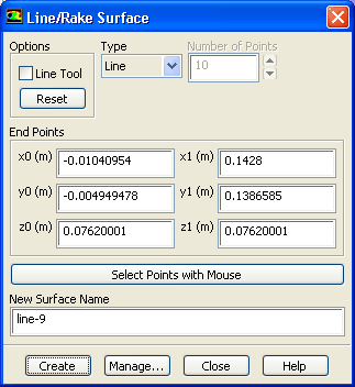
5.   Create a line surface from the center of wall-4 to the edge.

Surface $\rightarrow$ Line/Rake...

(a)   Enter the values for x0, x1, y0, y1, z0, and z1 as shown in the Line/Rake Surface dialog box.

  You can also select the points by clicking Select Points with Mouse. Then, in the graphic display, click at the center of wall-4 and at the edge using the right mouse button.

(b)   Click Create.

(c)   Close the Line/Rake Surface dialog box.

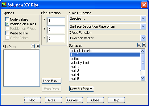
6.   Plot the surface deposition rate of Ga v/s radial distance (Figure  16.9).

Plots XY Plot Set Up...

(a)   Disable Node Values in the Options group box.

(b)   Select Species... and Surface Deposition Rate of ga from the Y Axis Function drop-down lists.

  The source/sink terms due to the surface reaction are deposited in the cell adjacent to the wall cells, so it is necessary to plot the cell values and not the node values.

(c)   Select line-9 from the Surfaces selection list.

(d)   Click Plot and close the Solution XY Plot dialog box.

  The peak surface deposition rate occurs at the center of wall-4 (where the concentration of the mixture is highest).

Figure 16.9: Plot of Surface Deposition Rate of Ga

Extra:    You can also perform all the postprocessing steps to analyze the deposition of As.

7.   Save the case and data files ( surface-react2.cas.gz and surface-react2.dat.gz).

File $\rightarrow$ Write $\rightarrow$ Case & Data...