Step 6: Initial Solution Without Droplets

  The airflow will first be solved and analyzed without droplets.

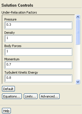
1.   Retain the default under-relaxation factors.

Solution Controls

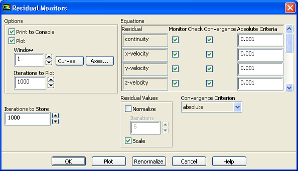
2.   Enable residual plotting during the calculation.

Monitors Residuals Edit...

(a)   Ensure that Plot is enabled in the Options group box.

(b)   Click OK to close the Residual Monitors dialog box.

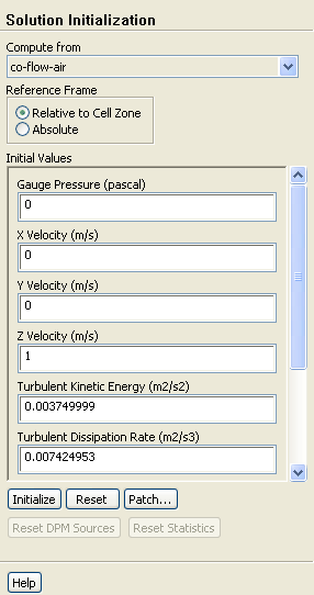
3.   Initialize the flow field.

Solution Initialization

(a)   Select co-flow-air from the Compute from drop-down list.

(b)   Click Initialize to initialize the variables.

4.   Save the case file ( spray1.cas.gz).

File $\rightarrow$ Write $\rightarrow$ Case...

5.   Start the calculation by requesting 300 iterations.

Run Calculation

(a)   Enter 300 for Number of Iterations.

(b)   Click Calculate.

  The solution will converge in approximately 250 iterations.

6.   Save the case and data files ( spray1.cas.gz and spray1.dat.gz).

File $\rightarrow$ Write $\rightarrow$ Case & Data...

Note:    ANSYS FLUENT will ask you to confirm that the previous case file is to be overwritten.

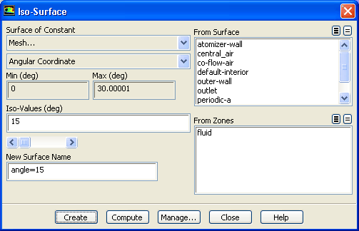
7.   Create a clip plane to examine the flow field at the midpoint of the atomizer section.

Surface $\rightarrow$ Iso-Surface...

(a)   Select Mesh... and Angular Coordinate from the Surface of Constant drop-down lists.

(b)   Click Compute to update the minimum and maximum values.

(c)   Enter 15 for Iso-Values.

(d)   Enter angle=15 for New Surface Name.

(e)   Click Create to create the isosurface.

(f)   Close the Iso-Surface dialog box.

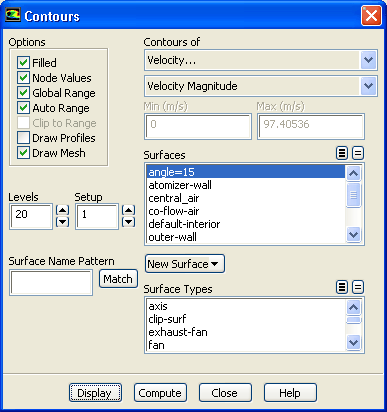
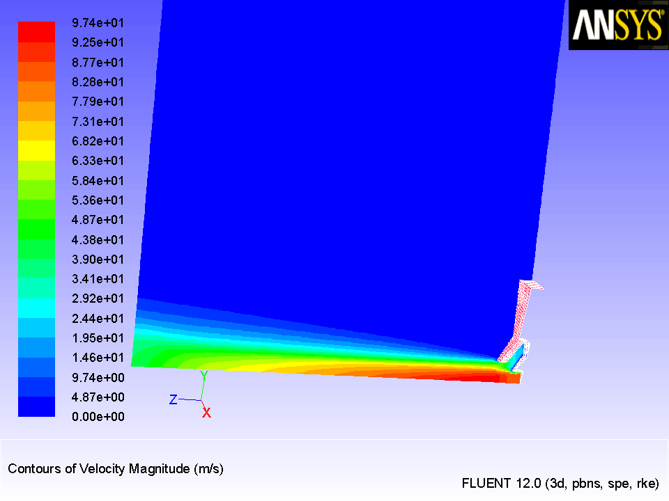
8.   Review the current state of the solution by examining contours of velocity magnitude (Figure  17.3).

Graphics and Animations Contours Set Up...

(a)   Enable Filled in the Options group box

(b)   Select Velocity... and Velocity Magnitude from the Contours of drop-down lists.

(c)   Enable Draw Mesh.

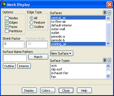
  The Mesh Display dialog box will open.

i.   Retain the current mesh display settings.

ii.   Close the Mesh Display dialog box.

(d)   Select angle=15 from the Surfaces selection list.

(e)   Click Display and close the Contours dialog box.

(f)   Use the mouse to obtain the view shown in Figure  17.3.

Figure 17.3: Velocity Magnitude at Mid-Point of Atomizer Section

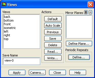
9.   Modify the view to include the entire atomizer.

Graphics and Animations Views...

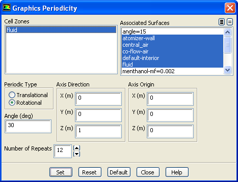
(a)   Click the Define... button to open the Graphics Periodicity dialog box.

i.   Select fluid from the Cell Zones selection list.

ii.   Retain the selection of Rotational in the Periodic Type list.

iii.   Retain the value of 12 for Number of Repeats.

iv.   Click Set and close the Graphics Periodicity dialog box.

  The graphics display will be updated to show the entire atomizer.

(b)   Click Apply and close the Views dialog box.

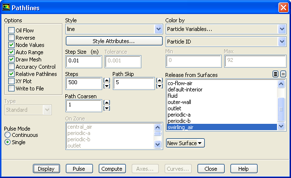
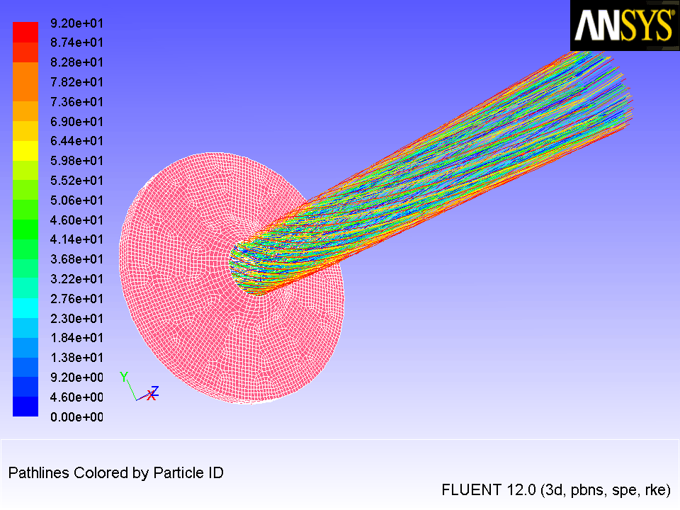
10.   Display pathlines of the air in the swirling annular stream (Figure  17.4).

Graphics and Animations Pathlines Set Up...

(a)   Increase the Path Skip value to 5.

(b)   Select swirling_air from the Release from Surfaces selection list.

  You will need to scroll down the list to access this item.

(c)   Enable Draw Mesh in the Options group box.

  The Mesh Display dialog box will open.

i.   Retain the current mesh display settings.

ii.   Close the Mesh Display dialog box.

(d)   Click Display and close the Pathlines dialog box.

(e)   Use the mouse to obtain the view shown in Figure  17.4.

Figure 17.4: Pathlines of Air in the Swirling Annular Stream