Step 8: Solution

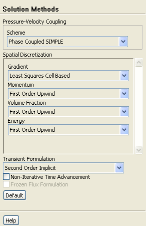
1.   Select the second order implicit transient formulation.

Solution Methods

(a)   Select Second Order Implicit from the Transient Formulation drop-down list.

(b)   Retain the default settings in the Spatial Discretization group box.

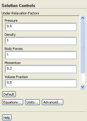
2.   Set the solution parameters.

Solution Controls

(a)   Enter 0.5 for Pressure.

(b)   Enter 0.2 for Momentum.

3.   Ensure that the plotting of residuals is enabled during the calculation.

Monitors Residuals Edit...

4.   Define a custom field function for the heat transfer coefficient.

Define $\rightarrow$ Custom Field Functions...

  Initially, you will define functions for the mixture temperature, and thermal conductivity, then you will use these to define a function for the heat transfer coefficient.

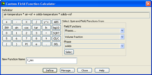
(a)   Define the function t_mix.

i.   Select Temperature... and Static Temperature from the Field Functions drop-down lists.

ii.   Ensure that air is selected from the Phase drop-down list and click Select.

iii.   Click the multiplication symbol in the calculator pad.

iv.   Select Phases... and Volume fraction from the Field Functions drop-down list.

v.   Ensure that air is selected from the Phase drop-down list and click Select.

vi.   Click the addition symbol in the calculator pad.

vii.   Similarly, add the term solids-temperature * solids-vof.

viii.   Enter t_mix for New Function Name.

ix.   Click Define.

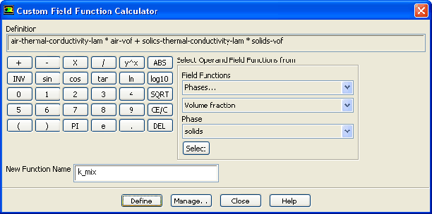
(b)   Define the function k_mix.

i.   Select Properties... and Thermal Conductivity from the Field Functions drop-down lists.

ii.   Select air from the Phase drop-down list and click Select.

iii.   Click the multiplication symbol in the calculator pad.

iv.   Select Phases... and Volume fraction from the Field Functions drop-down lists.

v.   Ensure that air is selected from the Phase drop-down list and click Select.

vi.   Click the addition symbol in the calculator pad.

vii.   Similarly, add the term solids-thermal-conductivity-lam * solids-vof.

viii.   Enter k_mix for New Function Name.

ix.   Click Define.

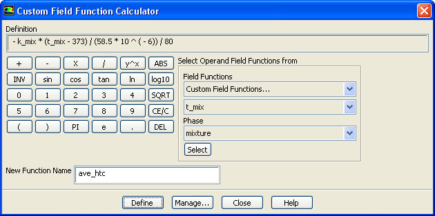
(c)   Define the function ave_htc.

i.   Click the subtraction symbol in the calculator pad.

ii.   Select Custom Field Functions... and k_mix from the Field Functions drop-down lists.

iii.   Use the calculator pad and the Field Functions lists to complete the definition of the function.

$- k\_mix \times (t\_mix - 373) / (58.5 \times 10^{(-6)}) / 80$

iv.   Enter ave_htc for New Function Name.

v.   Click Define and close the Custom Field Function Calculator dialog box.

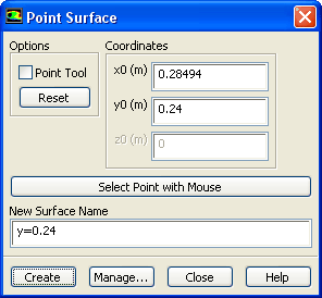
5.   Define the point surface in the cell next to the wall on the plane $y = 0.24$.

Surface $\rightarrow$ Point...

(a)   Enter 0.28494 m for x0 and 0.24 m for y0 in the Coordinates group box.

(b)   Enter y=0.24 for New Surface Name.

(c)   Click Create and close the Point Surface dialog box.

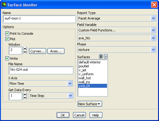
6.   Define a surface monitor for the heat transfer coefficient.

Monitors ( Surface Monitors) Create...

(a)   Enable Plot, and Write for surf-mon-1.

(b)   Enter htc-024.out for File Name.

(c)   Select Flow Time from the X Axis drop-down list.

(d)   Select Time Step from the Get Data Every drop-down list.

(e)   Select Facet Average from the Report Type drop-down list.

(f)   Select Custom Field Functions... and ave_htc from the Field Variable drop-down lists.

(g)   Select y=0.24 from the Surfaces selection list.

(h)   Click OK to close the Surface Monitor dialog box.

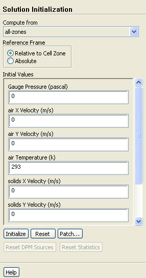
7.   Initialize the solution.

Solution Initialization

(a)   Select all-zones from the Compute from drop-down list.

(b)   Retain the default values and click Initialize.

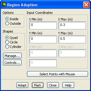
8.   Define an adaption register for the lower half of the fluidized bed.

Adapt $\rightarrow$ Region...

  This register is used to patch the initial volume fraction of solids in the next step.

(a)   Enter 0.3 m for Xmax and 0.5 m for Ymax in the Input Coordinates group box.

(b)   Click Mark.

(c)   Click the Manage... button to open the Manage Adaption Registers dialog box.

i.   Ensure that hexahedron-r0 is selected from the Registers selection list.

ii.   Click Display and close the Manage Adaption Registers dialog box.

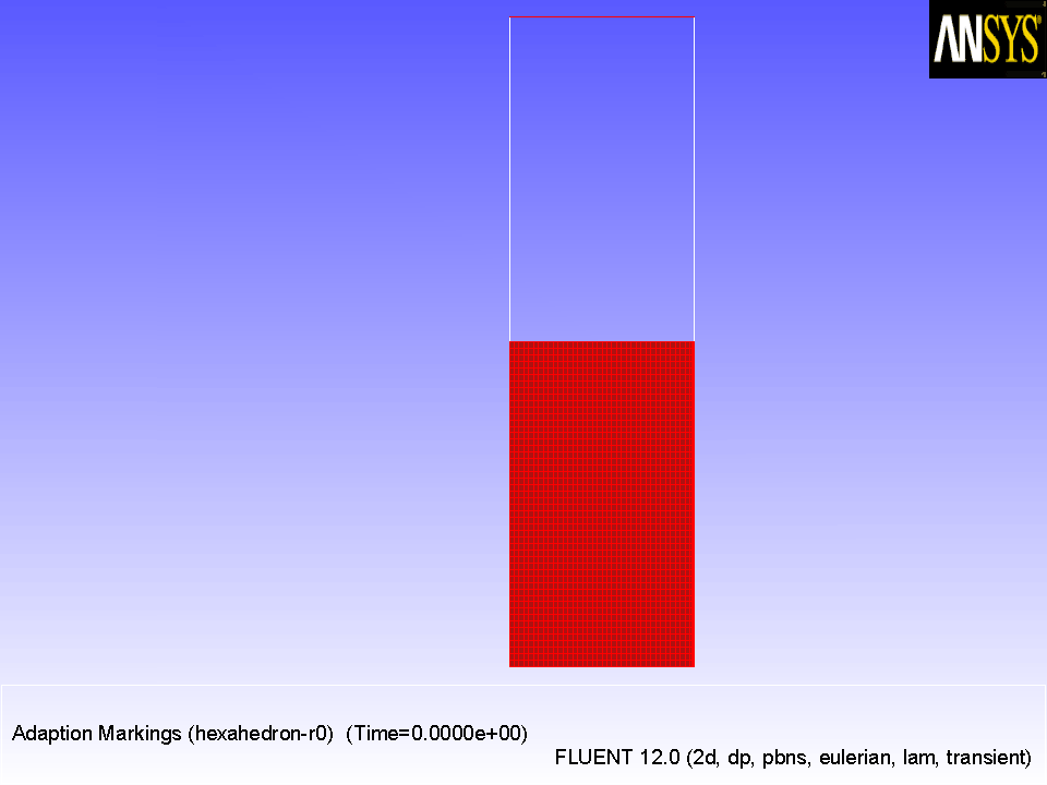
  After you define a region for adaption, it is a good practice to display it to visually verify that it encompasses the intended area.

Figure 23.3: Region Marked for Patching

(d)   Close the Region Adaption dialog box.

9.   Patch the initial volume fraction of solids in the lower half of the fluidized bed.

Solution Initialization Patch...

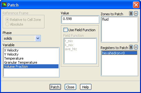
(a)   Select solids from the Phase drop-down list.

(b)   Select Volume Fraction from the Variable selection list.

(c)   Enter 0.598 for Value.

(d)   Select hexahedron-r0 from the Registers to Patch selection list.

(e)   Click Patch and close the Patch dialog box.

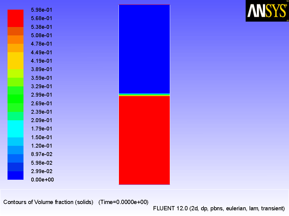
  At this point, it is a good practice to display contours of the variable you just patched, to ensure that the desired field was obtained.

10.   Display contours of Volume Fraction of solids (Figure  23.4).

Graphics and Animations Contours Set Up...

(a)   Enable Filled in the Options group box.

(b)   Select Phases... from the upper Contours of drop-down list.

(c)   Select solids from the Phase drop-down list.

(d)   Ensure that Volume fraction is selected from the lower Contours of drop-down list.

(e)   Click Display and close the Contours dialog box.

Figure 23.4: Initial Volume Fraction of Granular Phase (solids).

11.   Save the case file ( fluid-bed.cas.gz).

File $\rightarrow$ Write $\rightarrow$ Case...

12.   Set a time step size of 0.00025 s and run the calculation for 7000 time steps.

Run Calculation

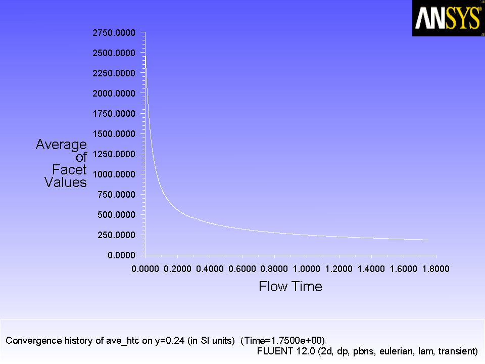
  The plot of the value of the mixture-averaged heat transfer coefficient in the cell next to the heated wall versus time is in excellent agreement with results published for the same case [1].

Figure 23.5: Plot of Mixture-Averaged Heat Transfer Coefficient in the Cell Next to the Heated Wall Versus Time

13.   Save the case and data files ( fluid-bed.cas.gz and fluid-bed.dat.gz).

File $\rightarrow$ Write $\rightarrow$ Case & Data...