Step 12: XY Plots

  XY plotting can be used to display quantitative results of your CFD simulations. Here, you will complete the review of the module cooling simulation by plotting the temperature distribution along the top centerline of the module.

1.   Define the line along which to plot results.

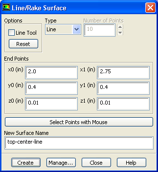
Surface $\rightarrow$ Line/Rake...

(a)   Select Line from the Type drop-down list.

(b)   Enter the coordinates of the line using a starting coordinate of ( 2.0, 0.4, 0.01) and an ending coordinate of ( 2.75, 0.4, 0.01).

  These coordinates define the top centerline of the module.

(c)   Enter top-center-line for New Surface Name.

(d)   Click Create and close the Line/Rake Surface dialog box.

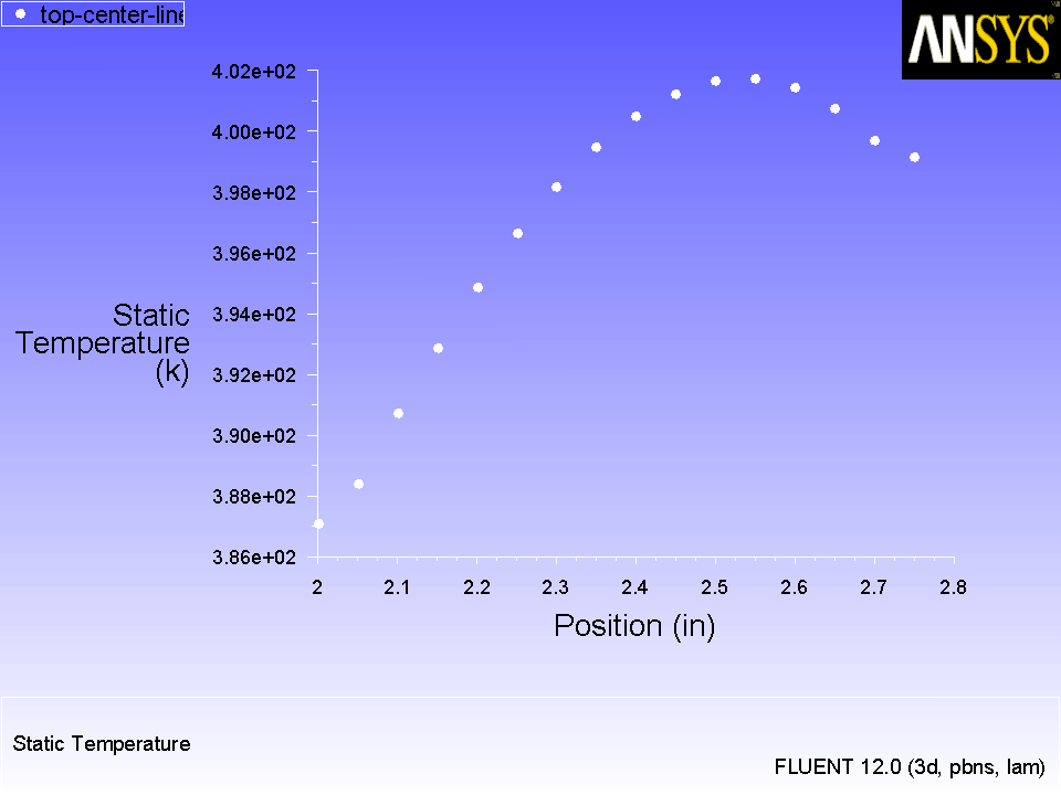
2.   Plot the temperature distribution along the top centerline of the module (Figure  24.20).

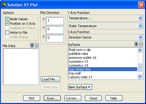
Plots XY Plot Set Up...

(a)   Retain the default Plot Direction of X.

(b)   Select Temperature... and Static Temperature from the Y Axis Function drop-down lists.

(c)   Select top-center-line from the Surfaces selection list.

  This will plot temperature vs the $x$ coordinate along the selected line ( top-center-line).

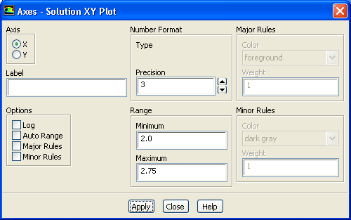
(d)   Click the Axes... button to open the Axes - Solution XY Plot dialog box.

i.   Retain the selection of X in the Axis list.

ii.   Disable Auto Range in the Options group box.

iii.   Enter 2.0 for Minimum and 2.75 for Maximum in the Range group box.

iv.   Click Apply and close the Axes - Solution XY Plot dialog box.

(e)   Click Plot and close the Solution XY Plot dialog box.

  The temperature distribution (Figure  24.20) shows the temperature increase across the module surface as the thermal boundary layer develops in the cooling air flow.

Figure 24.20: Temperature Along the Top Centerline of the Module