Step 5: Contours

Graphics and Animations Contours Set Up...

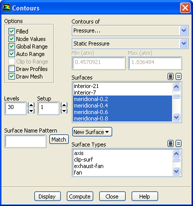
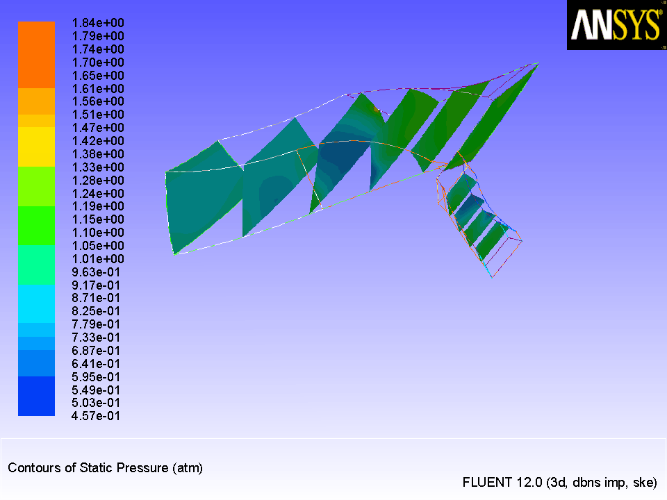
1.   Display filled contours of pressure on the meridional isosurfaces (Figure  25.2).

(a)   Make sure Filled is enabled in the Options group box.

(b)   Retain the selection of Pressure... and Static Pressure from the Contours of drop-down lists.

(c)   Select rotor-inlet, meridional-0.2, meridional-0.4, meridional-0.6, meridional-0.8, and rotor-outlet from the Surfaces selection list.

(d)   Enable Draw Mesh in the Options group box.

  The Mesh Display dialog box will open.

i.   Retain the current settings and close the Mesh Display dialog box.

(e)   Click Display.

(f)   Rotate and zoom the display using the left and middle mouse buttons, respectively, to obtain the view shown in Figure  25.2.

  In Figure  25.2, you can observe the buildup of static pressure along the duct.

Figure 25.2: Filled Contours of Pressure on the Meridional Isosurfaces

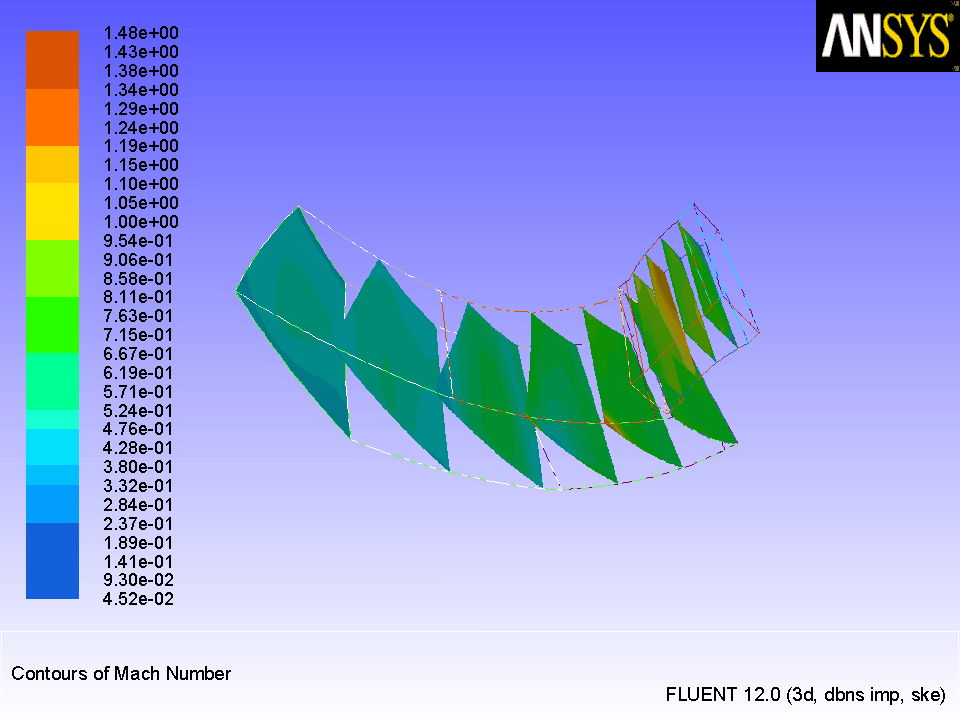
2.   Display filled contours of Mach number (Figure  25.3).

(a)   Select Velocity... and Mach Number from the Contours of drop-down lists.

(b)   Click Display.

  In Figure  25.3, you can observe locations at which the flow becomes slightly supersonic, about halfway through the duct.

Figure 25.3: Filled Contours of Mach Number on the Meridional Isosurfaces

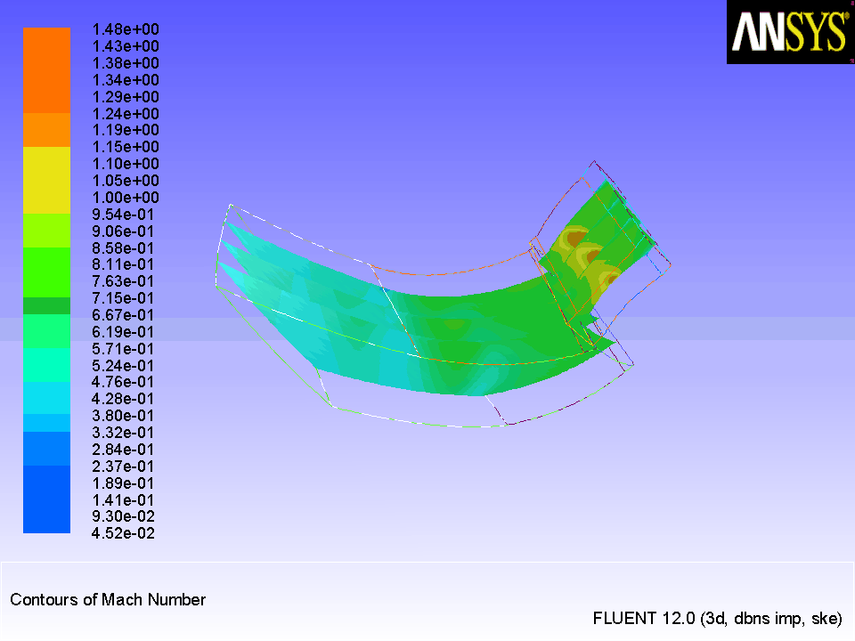
3.   Display filled contours of Mach number on the spanwise isosurfaces (Figure  25.4).

(a)   Deselect all surfaces in the Surfaces selection list.

(b)   Select spanwise-0.25, spanwise-0.5, and spanwise-0.75 from the Surfaces selection list.

(c)   Click Display.

  The display in Figure  25.4 allows you to further study the variation of the Mach number inside the duct. You may want to explore using different combinations of surfaces to display the same or additional variables.

Figure 25.4: Filled Contours of Mach Number on the Spanwise Isosurfaces

4.   Display a 360-degree image of the Mach number contours on the hub and blade wall surfaces.

(a)   Deselect all surfaces in the Surfaces selection list.

(b)   Select rotor-hub, rotor-blade-pressure and rotor-blade-suction from the Surfaces selection list.

(c)   Click Display.

(d)   Display the full 360-degree geometry.

Graphics and Animations Views...

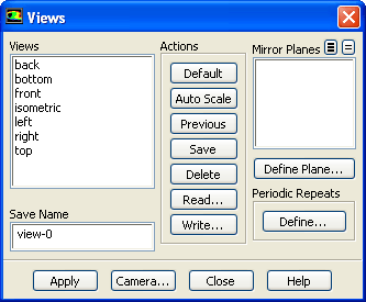
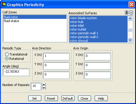
i.   Click the Define... button to open the Graphics Periodicity dialog box.

a.   Select fluid-rotor in the Cell Zones list.

  This will select all the surfaces in the Associated Surfaces list. The default value for Number of Repeats is set to 16. The display is updated to give a full, 360 degree view.

b.   Click Set and close the Graphics Periodicity dialog box.

  The display will be updated to show the entire geometry (see Figure  25.5).

Figure 25.5: Filled Contours of Mach Number on the 0.5 Spanwise Isosurface

ii.   Close the Views dialog box.

5.   Close the Contours dialog box.

Note:   This step demonstrated a typical view-manipulation task. See Tutorial 24 for further examples of postprocessing features.