[ANSYS, Inc. Logo] return to home search
next up previous contents

Step 2: Reading and Partitioning the Mesh

  When you use the parallel solver, you need to subdivide (or partition) the mesh into groups of cells that can be solved on separate processors. If you read an unpartitioned mesh into the parallel solver, ANSYS FLUENT will automatically partition it using the default partition settings. You can then check the partitions to see if you need to modify the settings and repartition the mesh.

1.   Inspect the automatic partitioning settings.

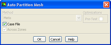
Parallel $\rightarrow$ Auto Partition...

figure

  If the Case File option is enabled (the default setting), and there exists a valid partition section in the case file (i.e., one where the number of partitions in the case file divides evenly into the number of compute nodes), then that partition information will be used rather than repartitioning the mesh. You need to disable the Case File option only if you want to change other parameters in the Auto Partition Mesh dialog box.

(a)   Retain the Case File option.

  When the Case File option is enabled, ANSYS FLUENT will automatically select a partitioning method for you. This is the preferred initial approach for most problems. In the next step, you will inspect the partitions created and be able to change them, if required.

(b)   Click OK to close the Auto Partition Mesh dialog box.

2.   Read the case file elbow3.cas.gz.

File $\rightarrow$ Read $\rightarrow$ Case...

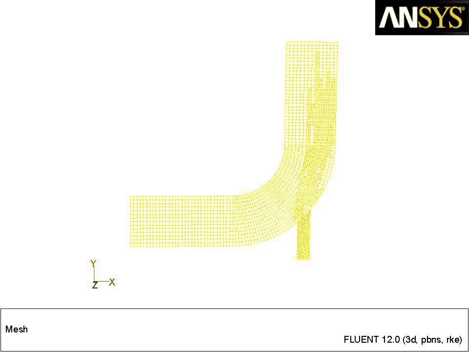
3.   Examine the front view of the symmetry mesh zone (Figure  26.2).

Note:   Since the Display Options were enabled by default in the launcher, the mesh was displayed in the embedded graphics window after reading in the case.

Figure 26.2: Mesh Along the Symmetry Plane for the Mixing Elbow
figure

4.   Check the partition information.

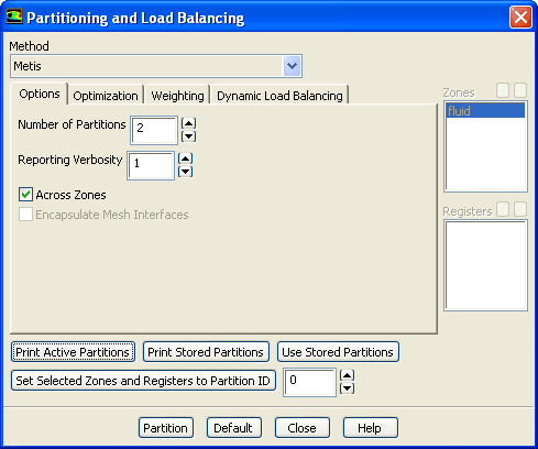
Parallel $\rightarrow$ Partitioning and Load Balancing...

figure

(a)   Click Print Active Partitions.

   ANSYS FLUENT will print the active partition statistics in the console.

>> 2 Active Partitions:
    P   Cells I-Cells Cell Ratio   Faces I-Faces Face Ratio Neighbors Load
    0   10414     177      0.017   34000     209      0.006         1    1
    1   10417     173      0.017   34646     209      0.006         1    1

   ----------------------------------------------------------------------
   Collective Partition Statistics:        Minimum   Maximum   Total     
   ----------------------------------------------------------------------
   Cell count                              10414     10417     20831     
   Mean cell count deviation               -0.0\%     0.0\%      
   Partition boundary cell count           173       177       350       
   Partition boundary cell count ratio     1.7\%      1.7\%      1.7\%      

   Face count                              34000     34646     68437     
   Mean face count deviation               -0.9\%     0.9\%      
   Partition boundary face count           209       209       209       
   Partition boundary face count ratio     0.6\%      0.6\%      0.3\%      

   Partition neighbor count                1         1         
   ----------------------------------------------------------------------
   Partition Method                        Metis                                
   Stored Partition Count                  2                                    
Done.

Note:    ANSYS FLUENT distinguishes between two cell partition schemes within a parallel problem--the active cell partition, and the stored cell partition. Here, both are set to the cell partition that was created upon reading the case file. If you repartition the mesh using the Partition Mesh dialog box, the new partition will be referred to as the stored cell partition. To make it the active cell partition, you need to click the Use Stored Partitions button in the Partition Mesh dialog box. The active cell partition is used for the current calculation, while the stored cell partition (the last partition performed) is used when you save a case file. This distinction is made mainly to allow you to partition a case on one machine or network of machines and solve it on a different one.

For details, see this chapter in the separate User's Guide.

(b)   Review the partition statistics.

  An optimal partition should produce an equal number of cells in each partition for load balancing, a minimum number of partition interfaces to reduce interpartition communication bandwidth, and a minimum number of partition neighbors to reduce the startup time for communication. Here, you will be looking for relatively small values of mean cell and face count deviation, and total partition boundary cell and face count ratio.

(c)   Close the Partitioning and Load Balancing dialog box.

5.   Examine the partitions graphically.

(a)   Initialize the solution using the default values.

figure Solution Initialization figure Initialize

  In order to use the Contours dialog box to inspect the partition you just created, you have to initialize the solution, even though you are not going to solve the problem at this point. The default values are sufficient for this initialization.

(b)   Display the cell partitions (Figure  26.3).

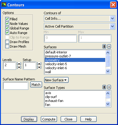
figure Graphics and Animations figure figure Contours figure Set Up...

figure

i.   Make sure Filled is enabled in the Options group box.

ii.   Select Cell Info... and Active Cell Partition from the Contours of drop-down lists.

iii.   Select symmetry from the Surfaces selection list.

iv.   Set Levels to 2, which is the number of compute nodes.

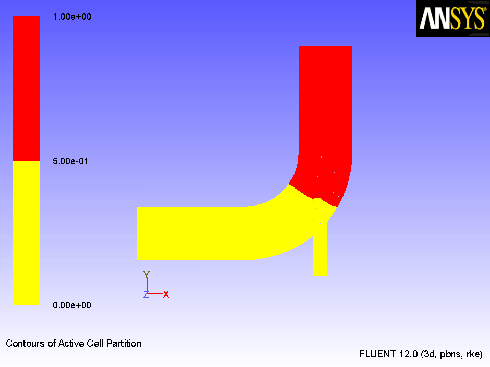
v.   Click Display and close the Contours dialog box.

Figure 26.3: Cell Partitions
figure

  As shown in Figure  26.3, the cell partitions are acceptable for this problem. The position of the interface reveals that the criteria mentioned earlier will be matched. If you are dissatisfied with the partitions, you can use the Partition Mesh dialog box to repartition the mesh. Recall that, if you wish to use the modified partitions for a calculation, you will need to make the Stored Cell Partition the Active Cell Partition by either clicking the Use Stored Partitions button in the Partition Mesh dialog box, or saving the case file and reading it back into ANSYS FLUENT.

For details about the procedure and options for manually partitioning a mesh, see this section in the separate User's Guide.

6.   Save the case file with the partitioned mesh ( elbow4.cas.gz).

File $\rightarrow$ Write $\rightarrow$ Case...


next up previous contents Previous: Step 1B: Network of
Up: Parallel Processing
Next: Step 3: Solution
Release 12.0 © ANSYS, Inc. 2009-02-09