3.3.1 Enabling the Population Balance Model

The procedure for setting up a population balance problem is described below. (Note that this procedure includes only those steps necessary for the population balance model itself; you will need to set up other models, boundary conditions, etc. as usual. See the ANSYS FLUENT User's Guide for details.)

1.   Start the double-precision version of ANSYS FLUENT.

2.   To enable the population balance model, follow the instructions in Section  3.2.

Remember to enable the mixture or Eulerian multiphase model.

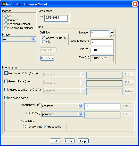
3.   Open the Population Balance Model dialog box (Figure  3.3.1).

Models Population Balance Edit...

Figure 3.3.1: The Population Balance Model Dialog Box

4.   Specify the population balance method under Method.

• If you select Discrete, you will need to specify the following parameters:

  Definition   can be specified as a Geometric Ratio or as a File. If Geometric Ratio is selected, then the Ratio Exponent must be specified. If File is selected, you will click the Load File... button and select the bin size file that you want loaded.

  You can input the diameter through the text file, with each diameter listed on a separate line, starting from the largest to the smallest diameter. Hence, you are not limited by the choices specified in the dialog box.

  Number   specifies the number of particle size bins used in the calculation.

  Ratio Exponent   specifies the exponent $q$ used in the discretization of the growth term volume coordinate (see Section  2.3.1).

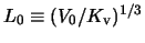
  Min   specifies the minimum bin size $L_0 \equiv (V_0/K_{\rm v})^{1/3}$.

  Max   displays the maximum bin size, which is calculated internally.

  Kv   specifies the value for the particle volume coefficient $K_{\rm v}$ (as described in Section  2.2.1). By default, this coefficient has a value of $\pi/6$.

  To display a list of the bin sizes in the console window, click Print Bins. The bin sizes will be listed in order of size, from the largest to the smallest. This option is only available when the Geometric Ratio Definition is selected.

• If you select Standard Moment under Method, you will specify the number of Moments under Parameters.

• If you selected Quadrature Moment under Method, you will set the number of moments to either 4, 6 or 8 under Parameters.

5.   Select the secondary phase from the Phase drop-down list for which you want to apply the population balance model parameters.

6.   For all population balance methods, you can enable the following under Phenomena:

Nucleation Rate   allows you to specify the nucleation rate (particles/m $^3$-s). You can select constant or user-defined from the drop-down list. If you select constant, specify a value in the adjacent field. If you have a user-defined function (UDF) that you want to use to model the nucleation rate, you can choose the user-defined option and specify the appropriate UDF.

Growth Rate   allows you to specify the particle growth rate (m/s). You can select constant or user-defined from the drop-down list. If you select constant, specify a value in the adjacent field. If you have a user-defined function (UDF) that you want to use to model the growth rate, you can choose the user-defined option and specify the appropriate UDF.

Aggregation Kernel   allows you to specify the aggregation kernel (m $^3$/s). You can select constant, luo-model, free-molecular-model, turbulent-model, or user-defined from the drop-down list:

• If you select constant, specify a value in the adjacent field.

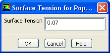
• If you select luo-model, the Surface Tension for Population Balance dialog box will open automatically to allow you to specify the surface tension (see Figure  3.3.2). The aggregation rate for the model will then be calculated based on Luo's aggregation kernel (as described in Section  2.2.2).

  Figure 3.3.2: The Surface Tension for Population Balance Dialog Box

  

• If you select free-molecular-model, then Equation  2.2-33 is applied.

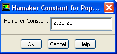
• If you select turbulent-model, the Hamaker Constant for Population Balance dialog box will open automatically to allow you to specify the Hamaker constant (see Figure  3.3.3). More information about this model is available in Section  2.2.2.

  Figure 3.3.3: The Hamaker Constant for Population Balance Dialog Box

  

• If you have a user-defined function (UDF) that you want to use to model the aggregation rate, you can choose the user-defined option and specify the appropriate UDF.

Breakage Kernel   allows you to specify the particle breakage frequency (particles/m $^3$-s). You can select constant, luo-model, lehr-model, ghadiri-model, or user-defined from the Frequency drop-down list:

• If you select constant, specify a value in the adjacent field.

• If you select luo-model, the Surface Tension for Population Balance dialog box will open automatically to allow you to specify the surface tension (see Figure  3.3.2). The frequency used in the breakage rate will then be calculated based on Luo's breakage kernel (as described in Section  2.2.2).

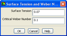
• If you select lehr-model, the Surface Tension and Weber Number dialog box will open automatically to allow you to specify the surface tension and critical Weber number (see Figure  3.3.4). The frequency used in the breakage rate will then be calculated based on Lehr's breakage kernel (as described in Section  2.2.2).

  Figure 3.3.4: The Surface Tension and Weber Number Dialog Box

  

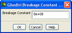
• If you select ghadiri-model, the Ghadiri Breakage Constant for Population Balance dialog box will open automatically to allow you to specify the breakage constant (see Figure  3.3.5). The frequency will then be calculated based on Ghadiri's breakage kernel (as described in Section  2.2.2).

  Figure 3.3.5: The Ghadiri Breakage Constant for Population Balance Dialog Box

  

• If you have a user-defined function (UDF) that you want to use to model the frequency for the breakage rate, you can choose the user-defined option and specify the appropriate UDF.

If you selected constant, ghadiri-model, or user-defined for Frequency, then you can specify the probability density function used to calculate the breakage rate by making a selection in the PDF drop-down list. You can select parabolic, generalized, or user-defined:

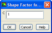
• If you select parabolic, the Shape Factor for Parabolic PDF dialog box will open automatically to allow you to specify the shape factor C (see Figure  3.3.6). The PDF used in the breakage rate will then be calculated according to Equation  2.2-15 (as described in Section  2.2.2).

  Figure 3.3.6: The Shape Factor for Parabolic PDF Dialog Box

  

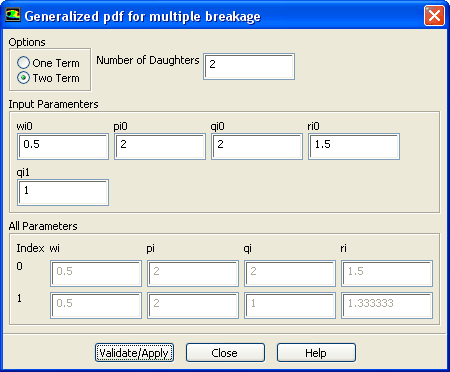
• If you select generalized, the Generalized pdf for multiple breakage dialog box will open automatically (Figure  3.3.7).

  Figure 3.3.7: The Generalized pdf for multiple breakage Dialog Box

  

  Perform the following steps in the Generalized pdf for multiple breakage dialog box:

  (a)   Select either One Term or Two Term from the Options list. Your selection will determine whether $i$ in Equation  2.2-21 is 0 or 1, respectively.

  (b)   Enter a value for the averaged Number of Daughters. It can be any real number (including non-integers, e.g., 2.5), as long as it is not less than 2.

  (c)   Define the parameter(s) for Equation  2.2-21 in the Input Parameters group box. When One Term is selected from the Options list, you must enter a value for qi0. When Two Term is selected from the Options list, you must enter values for wi0, pi0, qi0, ri0, and qi1. For information about appropriate values for these parameters to result in the daughter distributions shown in Table  2.2.2, see Table  2.2.3.

  (d)   Click the Validate/Apply button to save the settings. The text boxes in the All Parameters group box will be updated, using the values you entered in the Input Parameters group box, as well as values derived from the constraints shown in Equations  2.2-22- 2.2-24.

  (e)   Verify that the values in the All Parameters group box represent your intended PDF before clicking Close.

• If you have a user-defined function (UDF) that you want to use to model the PDF for the breakage rate, you can choose the user-defined option and specify the appropriate UDF. See Chapter  5 for details about UDFs for the population balance model.

Choose between the default Hagesather formulation and the Ramakrishna formulation. Detailed information about these two methods can be found in Section  2.3.1.

7.   Specify the boundary conditions for the solution variables.

Boundary Conditions

See Section  3.3.2 below.

8.   Specify the initial guess for the solution variables.

Solution Initialization

9.   Solve the problem and perform relevant postprocessing functions.

Run Calculation

See Chapter  4 for details about postprocessing.